Historical backend comparisons

This page preserves the earlier comparison with a 0.0625 Hz spherical cutoff and a 0.125 Hz QSEIS Nyquist limit. Its measurements, parameter scans and references to “current” examples describe that historical configuration, including the earlier SPGRN2012 effective source. Use the current comparison for the fresh 2 Hz / 1.25 s calculation, or the 64 s tutorial comparison for the later unified 0.125 Hz example protocol. Downloaded source helpers and reproduction scripts now contain the updated implementation; they are not archived historical scripts.

The SPGRN2012, SPGRN2020 and QSSP2020 examples use the same elastic model and source, but matching their named parameters alone does not produce equivalent numerical truncation. A controlled comparison found that the original low-cost SPGRN2020 and QSSP2020 settings retained too little low-frequency spatial content. Their files and array shapes were valid and their values finite, but their displacement waveforms differed substantially.

The current SPGRN2020 tutorial therefore uses max_slowness=0, and QSSP2020 uses min_harmonic=2000, max_harmonic=8000. These choices were checked for this example. They are not universal convergence settings or an absolute reference solution.

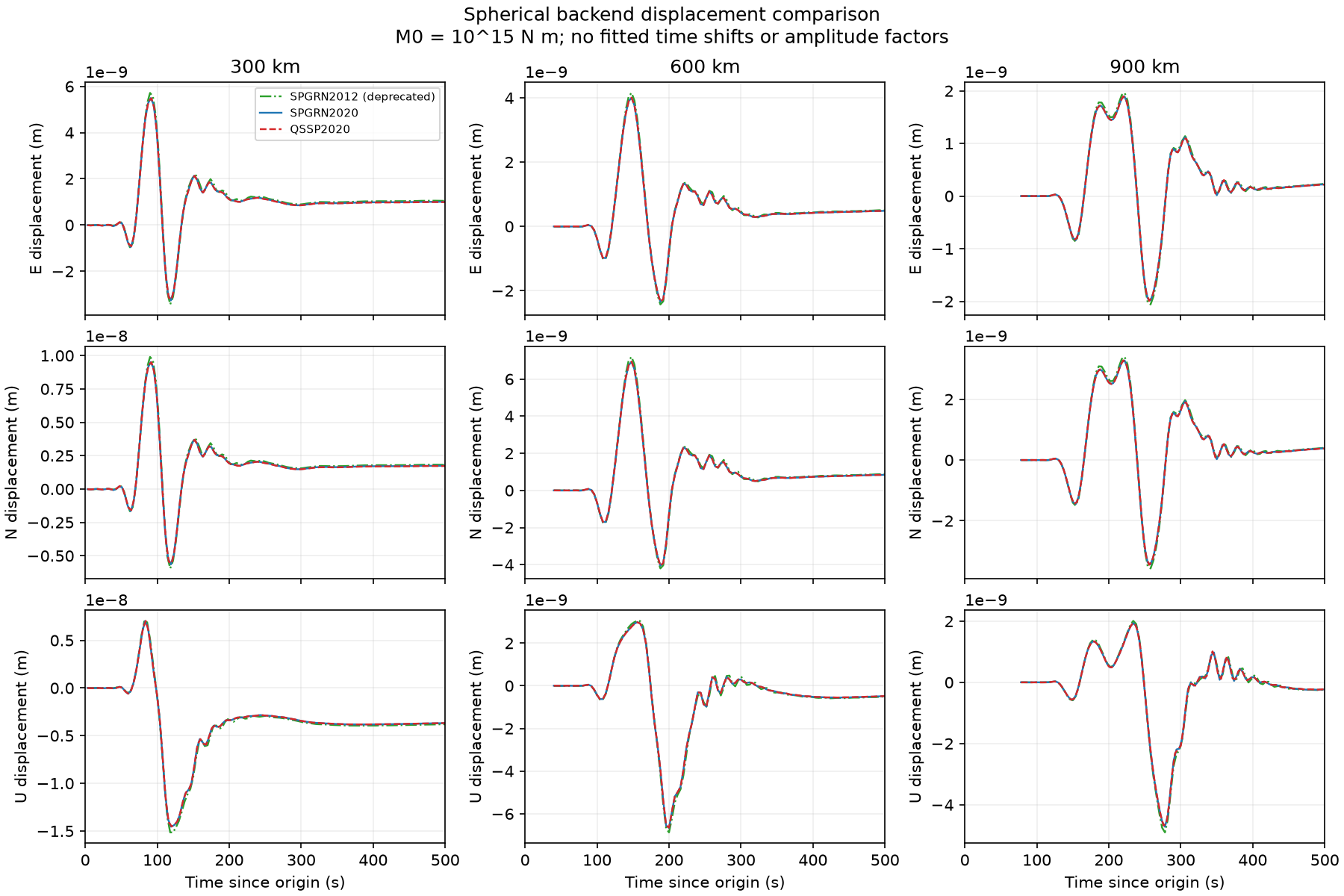
Three-component displacement at 300, 600 and 900 km. SPGRN2020 uses its full-wavefield branch and QSSP2020 uses the revised harmonic settings. All horizontal axes refer to source origin; their stored start times differ.

After running the three spherical examples and both QSEIS regional examples, generate comparisons from the completed libraries’ saved arrays:

python examples/compare_backends.py

The script uses the default example input directories and writes all-backends.png, spherical-comparison.png, qseis-comparison.png and comparison.json beneath examples/output/backend-comparison/. It compares physical times and reports differences without fitting a time shift or amplitude scale. It does not rerun solvers.

What the comparison holds fixed

The calculation uses the full bundled AK135 elastic model with constant Qp=600 and Qs=300, not the original AK135-F attenuation profile. The source is 10 km deep and receivers are at the surface, at 300, 600 and 900 km. Source strike/dip/rake are 30°/45°/90°, receiver azimuth is 30°, and scalar moment is 1e15 N m. Returned components are east, north and up, in metres.

All three use a 64 s squared half-sinusoid moment-rate pulse, a 4 s sample interval, 256 output samples, and a 0.0625 Hz frequency cutoff. The requested spectral window is 4092 s, giving a 4096 s FFT period; the output span is 1020 s. The anti-aliasing factor is 0.01. Spheroidal and toroidal modes are enabled, and self-gravitation and physical dispersion are disabled. The original positive slowness cutoff was 0.3 s/km in all three backends.

Align physical times before comparing arrays

The native sample starts, in seconds since source origin, are:

Backend	300 km	600 km	900 km
SPGRN2012	-10	20	50
SPGRN2020	3	40	78
QSSP2020	0	0	0

SPGRN2012 rounds t0 + distance / v0 to integer seconds. SPGRN2020 rounds the P onset minus green_before_p to integer seconds. For this example, its fractional P onsets are approximately 43.417, 80.497 and 117.540 s. The SPGRN2020 example uses the native binary header starts when saving and plotting times. A P-relative axis starting at -40 s, or simply adding those fractional P onsets, is different from the stored source-origin grid.

Use the common physical time interval when comparing traces. Do not compare sample indices across libraries or infer a 32 s source-centroid shift from the source duration.

Why the original harmonic settings differed

The original logs report these highest retained harmonic degrees:

Backend and original setting	At 0 Hz	At 0.015625 Hz	At 0.0625 Hz
SPGRN2012, slowness 0.3 s/km	504	566	751
SPGRN2020, slowness 0.3 s/km	54	242	804
QSSP2020, minimum 0 / maximum 800	12	196	750

A low temporal frequency can still require high spatial degrees, especially for shallow-source near-field displacement. Truncation can introduce spatial aliasing and distorted displacement baselines. The method and differential transformation are discussed by Wang et al. (2017).

For SPGRN2020, positive max_slowness uses the low-frequency baseline of 54 in this example; raising the cutoff from 0.3 to 1.0 s/km does not remove that limitation. A value of zero selects the full-wavefield branch, which starts from a baseline of 2500 and selects a model-dependent slowness limit. The actual maximum degree in the tested full-wavefield run was 3403. See the branch in qpmaxdeg.f and its constants in qpalloc.f.

For QSSP2020, min_harmonic controls the low-frequency baseline of the frequency-dependent upper degree, subject to the solver’s decay criterion. It does not exclude lower degrees: summation begins at zero. max_harmonic caps that upper degree. These operations appear in qpgrnspec.f.

QSSP maximum degree also affects synthesis

QSSP’s spatial differential-transformation order depends on the maximum degree allocated from max_harmonic. Let L_max denote that input parameter; the allocated maximum is L_max + 3. For this surface-receiver, 10 km source example, its threshold in radians is

\[ d_0=5\left(\frac{2\pi}{L_{\max}+3}+\frac{10}{6371}\right). \]

For angular distance d <= d_0 the order is zero. Otherwise it is min(2, trunc(log(d / d_0))), using the natural logarithm. This gives:

max_harmonic	Order at 300 km	Order at 600 km	Order at 900 km
800	0	0	1
1600	0	1	1
3200	0	1	2

The formula is specialized to this geometry; the full implementation also uses a path-depth measure. See qpwvint.f.

With min_harmonic=0, maximum settings 800, 1600 and 3200 produced eight corresponding GreenSpec files with identical SHA-256 hashes: the actual spectral upper degree remained 750. Nevertheless the synthesis order changed, and the waveforms changed at the affected distances. Similarly, with minimum 2000, raising the maximum from 3200 to 8000 left the spectra identical while changing the 300 km waveform by 23.68%. At finite truncation, changing the transformation and taper can alter the error. Increasing only the maximum need not improve the waveform monotonically.

Measured differences and scope

The following differences use SPGRN2020 with max_slowness=0 as the numerical reference. Each pair is compared from its latest native start time through 500 s, with linear interpolation onto a 1 s common grid. The metric is 100 * norm(u - u_ref) / norm(u_ref) across all three components. No amplitude fitting, time-shift fitting or baseline removal is applied; the reference is not treated as absolute truth.

Calculation setting	300 km	600 km	900 km
SPGRN2012, original	4.078%	4.403%	4.258%
SPGRN2020, slowness 0.3	42.406%	3.991%	2.331%
SPGRN2020, slowness 1.0	32.107%	2.327%	0.262%
QSSP, minimum 0 / maximum 800	179.242%	110.920%	16.750%
QSSP, 0 / 1600	179.242%	31.137%	16.750%
QSSP, 0 / 3200	179.242%	31.137%	112.873%
QSSP, 500 / 3200	484.041%	1.620%	2.329%
QSSP, 1000 / 3200	8.596%	0.378%	1.423%
QSSP, 2000 / 3200	19.109%	0.378%	1.423%
QSSP, 2000 / 8000	0.889%	0.378%	1.423%
QSSP, 4000 / 8000	0.890%	0.378%	1.423%

At a fixed maximum of 8000, increasing the minimum from 2000 to 4000 changes QSSP’s own traces by at most 0.0074% over the complete 0–1020 s window, comparing matching samples with the same relative-norm metric. Over each complete common window, QSSP 2000/8000 differs from SPGRN2020’s full-wavefield result by approximately 0.99%, 0.64% and 1.94%. This checks stability and cross-backend agreement for the stated geometry and frequency band; it does not validate arbitrary models or static limits.

These measurements include nine fresh parameter-variation builds: two SPGRN2020 and seven QSSP2020 runs, in addition to the original three examples. Download the comparison measurements and see validation for the execution environment and example checks.

Remaining differences

All three intended source pulses span 0–64 s; there is no seconds-versus- samples error in these spherical examples. SPGRN2020 and QSSP2020 evaluate the pulse spectrum at complex frequency, including the numerical damping term. SPGRN2012’s older routine uses only real frequency. After damping correction, the latter gives an effective pulse area of approximately 1.03672 for the stated settings, about 3.67% above unity. This is consistent with much of its roughly 4% residual amplitude difference, but does not establish that the entire residual has that cause. Compare SPGRN2012 wavelet.f and SPGRN2020 swavelet.f.

SPGRN readers integrate native velocity using cumsum * dt, while QSSP accumulates displacement inside Fortran from a zero initial value. Different output windows and sample grids can therefore introduce baseline and discrete-integration differences. The remaining 1–4% inter-backend differences have not been completely separated into causes.

Repeating the check for your model

Match the full model, attenuation, mechanism, units, source pulse, enabled physics and physical time coordinates. First compare exact library grid points without arrival adjustment or post-processing. Inspect the actual frequency-dependent degree limits in solver logs; input values alone do not describe the retained spectrum.

Vary both QSSP harmonic controls and use SPGRN2020’s full-wavefield branch as an additional comparison where appropriate. Test the time window, source duration and frequency range needed for your observations, including late-time displacement if it matters. Record changes in waveforms as well as runtime and storage.

Use fresh output directories and recalculate compatible spectra after changing these parameters. --reuse only rereads an existing library; it does not update its physical or numerical settings. Archive generated inputs and the model alongside the output, and report the parameter range that was actually checked.

QSEIS at the same regional distances

The QSEIS2025 regional example and QSEIS06 regional example also use 300, 600 and 900 km, with 64 s source support and 4 s sampling. They enable the flat-Earth transformation and retain their 24-row layered half-space model. Their saved 0–1020 s windows make regional phases easier to inspect alongside the spherical examples.

Matching the effective source time function

The current regional examples explicitly match the effective physical moment-rate pulse to the one used by SPGRN2020 and QSSP2020:

\[ r(t)=\frac{2}{T}\sin^2\left(\frac{\pi t}{T}\right), \qquad 0\leq t\leq T,\quad T=64\ {\rm s}, \]

with zero rate outside this interval. Its area is one and its centroid is 32 s. Matching the duration alone is insufficient: the built-in QSEIS pulse is transformed at real frequency, while SPGRN2020/QSSP2020 use complex frequency. In the previous regional calculation, the final QSEIS damping correction therefore increased the effective pulse area to approximately 1.03676 and shifted its centroid to 32.151 s.

The regional examples now select wavelet_type=0 and install a custom input block of 1024 equally spaced nodes:

\[ t_j=\frac{jT}{1023},\qquad w_j=r(t_j)\exp(2\pi f_i t_j),\qquad f_i=\frac{\ln(0.01)}{2\pi\,4092},\qquad j=0,\ldots,1023. \]

Since fi < 0, the exponential decreases the input samples. Do not renormalize these written samples: their area is approximately 0.9647094485. Fortran transforms their piecewise-linear interpolant at real frequency, and its subsequent multiplication by exp(-2*pi*fi*t) restores the intended physical rate. The result approximates the analytic complex-frequency pulse; it is not assumed identical merely because both inputs say 64 s.

The source-construction helper is source_time_function.py. It supplies the low-level sample block after normal preprocessing. Each new regional output directory contains source_time_function.npz and source_time_function.json; library/stf.json records the matching library source metadata and hashes. The NPZ preserves the node times, target rate, written input rate and reconstructed effective pulse, so the source check can be repeated independently of the waveform plots. At that time the ordinary package reader did not infer that a type-0 input was a moment-rate pulse or integrate it when asked for displacement. These examples explicitly read velo, strain_rate or stress_rate, then performed exactly one cumsum * dt to obtain displacement, strain or stress. The readers now integrate type 0 like type 1, and the current examples request those observables directly. The short near-distance examples retain their built-in type-2 source.

An independent reconstruction of Fortran’s piecewise-linear transform gives the following checks for the 1024-node pulse:

Check	Measured value
Time-domain relative L2 error against analytic r(t)	1.988e-6
Relative spectral L2 error, 0–0.0625 Hz	1.758e-6
Effective physical area	1.000000000412
Effective centroid	32.000000734 s

Both L2 checks pass the 1e-5 tolerance. The spectral comparison uses the analytic transform at f + i*fi, with the QSEIS damping frequency. No additional time shift or waveform amplitude fit is applied. The tolerance applies to the relative norm across the sampled spectrum; pointwise relative errors near spectral zeros can be larger.

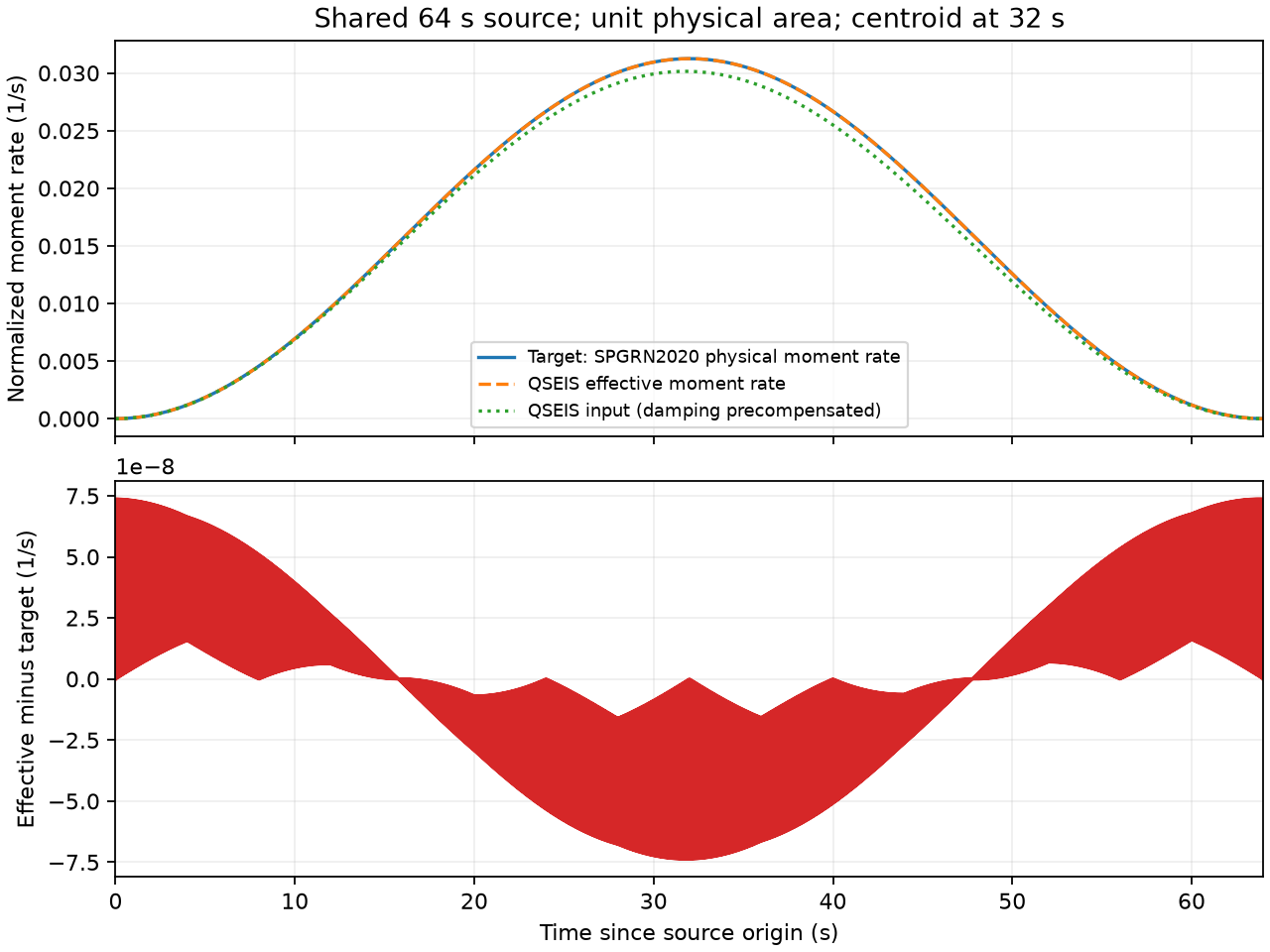
Physical moment-rate pulse and its numerical verification. The input samples include the damping compensation; the target physical area is one.

Download the source-time-function verification for the pulse checks and numerical settings.

Before matching the effective STF

The following historical results used the earlier QSEIS regional wavelet_type=2 pulse, before the damping compensation described above. They are not the results of the current custom-source example. The two QSEIS versions produced identical saved displacement samples in that run. Their differences relative to the SPGRN2020 full-wavefield example, on the same common time grid, were:

Backend before STF matching	300 km	600 km	900 km
QSEIS06	10.819%	17.516%	20.739%
QSEIS2025	10.819%	17.516%	20.739%

The corresponding combined ENU correlations were approximately 0.998, 0.994 and 0.991. These differences include the unmatched effective source pulse and other model/numerical effects. The source-area excess of about 3.68% alone does not establish the cause of the full 11–21% waveform discrepancy. The record before STF matching preserves that calculation separately from current results.

After matching the effective STF

Fresh runs with the compensated custom pulse gave the following comparison on exactly the same origin-time intervals, without fitting amplitudes or shifts:

QSEIS06 and QSEIS2025 versus SPGRN2020	300 km	600 km	900 km
Before matching the effective STF	10.819%	17.516%	20.739%
After matching the effective STF	12.684%	19.748%	22.951%

The two QSEIS versions again produced identical saved displacement samples. Their combined ENU correlations with SPGRN2020 after matching were 0.9978, 0.9935 and 0.9897. The shared pulse passes the independent area, centroid, time-shape and spectrum checks above, even though the seismogram differences increase. This controlled result rules out the previous STF mismatch as the main explanation of the 11–21% discrepancy: its excess amplitude had partly offset other waveform differences. No waveform was rescaled to force agreement. The remaining residuals have not been isolated into their separate physical and numerical contributions.

Remaining model and frequency differences

Matching the effective source does not make the physical models identical. The QSEIS model extends its bottom layer as a half-space, while the spherical model includes the complete Earth. The flat-Earth transformation does not restore the omitted deep structure.

Nor are the numerical frequency limits identical: at 4 s sampling, QSEIS evaluates frequencies up to the 0.125 Hz Nyquist limit and zeros the Nyquist bin, while the spherical examples impose a 0.0625 Hz cutoff. The 64 s source suppresses higher frequencies but is not strictly band-limited. Baseline and discrete-integration differences can also remain. The spherical harmonic-convergence percentages above do not include QSEIS.

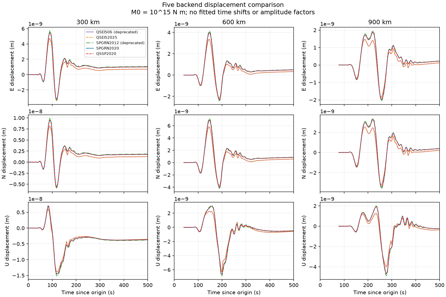
Comparison generated from the current example outputs over the common valid interval through 500 s. Each regional example separately exports 0–1020 s; physical source-origin times are used for the comparison.

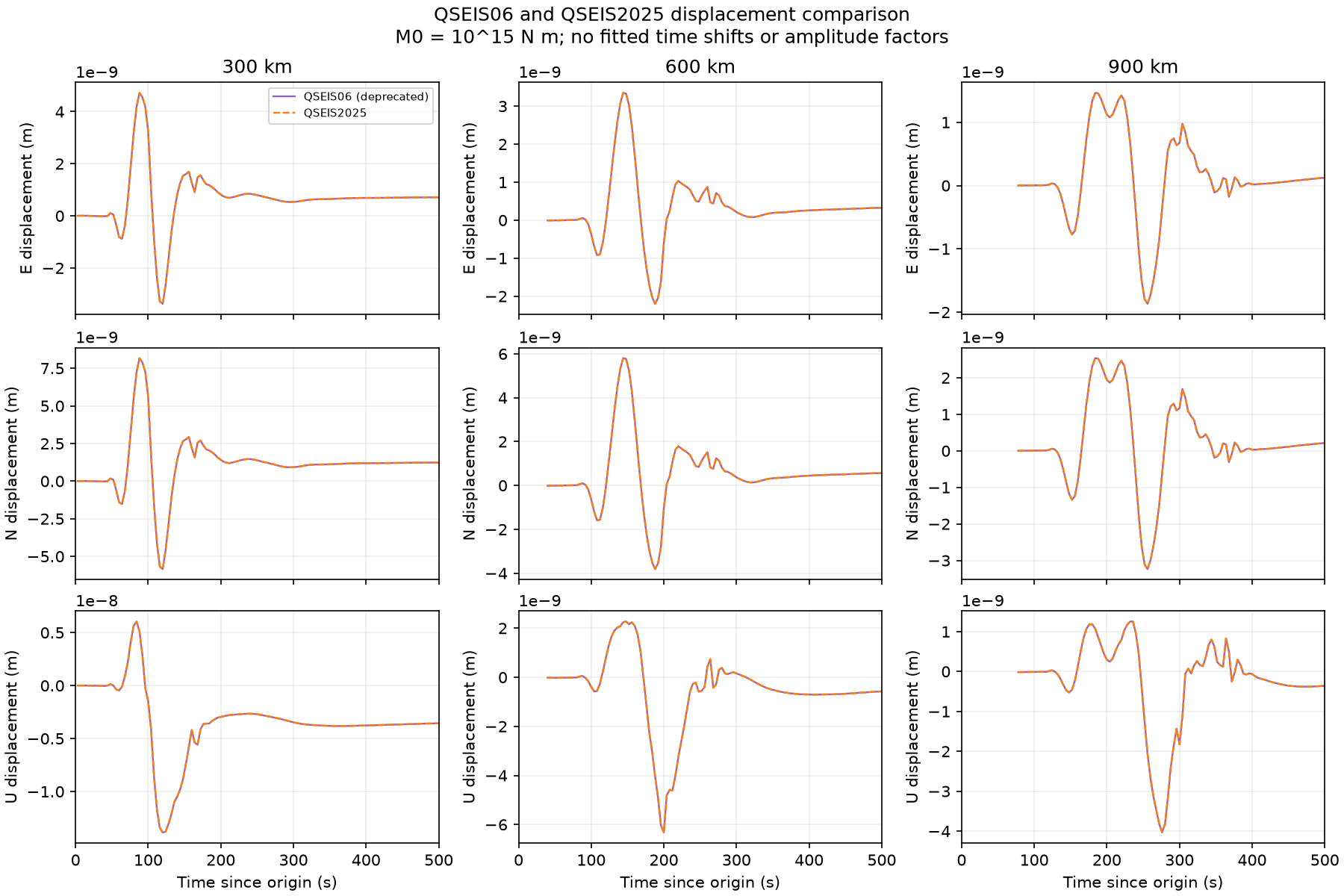
QSEIS06 and QSEIS2025 regional displacement on the same source-origin axis.

Download the five-backend record for per-component metrics, common time ranges, input hashes and model/parameter metadata. Run python examples/compare_backends.py after the five dynamic examples, including both QSEIS --regional commands, to regenerate the figures and checks. Its backend path options accept independent output directories.