QSEIS2025: displacement, strain and stress

QSEIS2025 calculates dynamic Green’s functions in a layered half-space and provides direct strain/stress and rotation kernels alongside vectors. Use this tutorial for a complete first calculation and for the introductory tensor workflow.

The fresh comparison dated 2026-09-15 adds five-backend displacement and QSEIS2025/QSSP2020 stress comparisons with 0.25 s sampling, a 2 Hz Nyquist limit, a 1.25 s effective source pulse and receivers 1 km deep. It also separates point-source results from the frequency-dependent Gaussian smoothing controls. The commands and figures below retain the 0–100 s introduction and the 64 s regional source with surface receivers; they do not generate that new comparison.

Build and inspect displacement

From the repository root:

python examples/qseis2025.py

The script prepares the model and input files, computes the library sequentially, reads three distances and saves an ENU displacement figure. E/N/U in example labels is the same east/north/up convention called ENZ by the API.

In the default near-distance mode, source depth is 10 km, receiver depth 0 km, and distances are 30, 60 and 90 km. The 0.5 s sample interval and 127.5 s window produce 256 native samples. After synthesis, every saved near-distance waveform and figure is cropped to 0–100 s inclusive (201 samples); the library keeps its full native window. The model uses the first 24 numeric rows and disables the flat-Earth transformation for this small half-space example. Moment is 10^15 N m.

Complete QSEIS2025 tutorial

"""Build QSEIS2025 introductory or regional traces; optionally include tensors."""
from pathlib import Path

from common import (MECHANISM, MOMENT_NM, REGIONAL_SAMPLING_INTERVAL_S, REGIONAL_STF, finish, parser_for, prepare,
                    require_library_settings, save_waveforms)
from pygrnwang.create_qseis2025_bulk import (
    pre_process_qseis2025, create_grnlib_qseis2025_sequential)
from pygrnwang.read_qseis2025 import get_outfile_name_list, seek_qseis2025
from source_time_function import prepare_qseis_stf, validate_qseis_stf
from spectral_settings import qseis_spectral_settings


def main():
    parser = parser_for("qseis2025")
    parser.add_argument("--regional", action="store_true",
                        help="Use 300/600/900 km, a 64 s wavelet and Earth flattening")
    parser.add_argument("--point-source", action="store_true",
                        help="Regional control run: disable the default Gaussian spatial source smoothing")
    parser.set_defaults(output_dir=None)
    parser.add_argument("--observables", choices=("disp", "all"), default="disp",
                        help="all also computes strain and stress")
    args = parser.parse_args()
    if args.point_source and not args.regional:
        parser.error("--point-source requires --regional")
    source_radius_ratio = 0.0 if args.point_source else 0.05
    if args.output_dir is None:
        directory = "qseis2025-regional" if args.regional else "qseis2025"
        if args.point_source:
            directory += "-point-source"
        args.output_dir = Path(__file__).resolve().parent / "output" / directory
    output, library, model, report, started = prepare(args, "QSEIS2025")
    dt, window = (REGIONAL_SAMPLING_INTERVAL_S, 4092.0) if args.regional else (0.5, 127.5)
    output_end = 1020.0 if args.regional else 100.0
    output_samples = int(round(output_end / dt)) + 1  # Include the final sample.
    native_samples = int(round(window / dt)) + 1
    distances = [300.0, 600.0, 900.0] if args.regional else [30.0, 60.0, 90.0]
    wavelet_duration = 16 if args.regional else 4
    wavelet_type = 0 if args.regional else 2
    source_time_function = None
    if not args.reuse:
        pre_process_qseis2025(
            processes_num=1, path_green=library, event_depth_list=[10.0],
            receiver_depth_list=[0.0], dist_range=[distances[0], distances[-1]],
            delta_dist=distances[0],
            N_each_group=3, time_window=window, sampling_interval=dt, source_radius_ratio=source_radius_ratio,
            output_observables=([1, 0, 1, 1, 0] if args.observables == "all"
                                else [1, 0, 0, 0, 0]),
            wavelet_type=wavelet_type, wavelet_duration=wavelet_duration, time_reduction_velo=0,
            flat_earth_transform=args.regional, path_nd=model, earth_model_layer_num=24,
        )
        if args.regional:
            source_time_function = prepare_qseis_stf(
                library, duration_s=64.0, samples=1024)
        create_grnlib_qseis2025_sequential(library, remove_pd=False)
    require_library_settings(
        library, event_depth_list=[10.0], receiver_depth_list=[0.0],
        grn_dist_range=[distances[0], distances[-1]], grn_delta_dist=distances[0],
        sampling_interval=dt, time_window=window, sampling_num=native_samples,
        wavelet_type=wavelet_type, wavelet_duration=wavelet_duration, time_reduction_velo=0,
        flat_earth_transform=args.regional, earth_model_layer_num=24,
        slowness_window=None, wavenumber_sampling_rate=12, anti_alias=0.01,
        free_surface=0,
    )
    native_input = Path(library) / "10.00" / "0.00" / "0_0" / "grn.inp"
    lines = native_input.read_text(encoding="utf-8-sig").splitlines()
    headings = [i for i, line in enumerate(lines) if "WAVENUMBER INTEGRATION PARAMETERS" in line]
    if len(headings) != 1:
        raise ValueError("Expected one native wavenumber section")
    data = [line.split("#", 1)[0].strip() for line in lines[headings[0] + 1:]]
    data = [line for line in data if line]
    controls = [float(value) for value in data[1].split()]
    if controls != [1e-6, source_radius_ratio]:
        raise ValueError("Existing native spatial-source settings differ; use a fresh --output-dir")
    if args.regional and args.reuse:
        source_time_function = validate_qseis_stf(library)
    observables = ("disp", "strain", "stress") if args.observables == "all" else ("disp",)
    if args.reuse:
        # Backend metadata does not store observable flags. Check the requested
        # binary outputs before reading a displacement-only library as tensors.
        native_dir = Path(library) / "10.00" / "0.00" / "0_0"
        required = []
        for observable in observables:
            psv, sh = get_outfile_name_list(observable)
            required.extend(native_dir / ("grn_%s.bin" % name) for name in psv + sh)
        if any(not path.is_file() for path in required):
            raise ValueError("Requested outputs are absent. Recalculate in a fresh "
                             "--output-dir without --reuse using --observables all.")
    for observable in observables:
        # Regional type-0 kernels are rates; the reader integrates them before cropping.
        arrays = [MOMENT_NM * seek_qseis2025(
            path_green=library, event_depth_km=10.0, receiver_depth_km=0.0,
            az_deg=30.0, dist_km=distance, focal_mechanism=MECHANISM,
            srate=1 / dt, output_type=observable, rotate=True,
            before_p=None, shift=False, pad_zeros=False,
        )[:, :output_samples] for distance in distances]
        labels = ["E", "N", "U"] if observable == "disp" else ["EE", "EN", "EU", "NN", "NU", "UU"]
        unit = {"disp": "m", "strain": "1", "stress": "Pa"}[observable]
        save_waveforms(output, report, observable, arrays, distances, dt, labels, unit,
                       expected_samples=output_samples, time_limits=(0.0, output_end))
    report.update(sampling_interval_s=dt, max_frequency_hz=0.5 / dt, time_window_s=window,
                  output_time_range_s=[0.0, output_end], distances_km=distances,
                  native_samples=native_samples, earth_model_numeric_rows=24,
                  wavelet_type=wavelet_type, wavelet_duration_samples=wavelet_duration,
                  wavelet_duration_s=wavelet_duration * dt,
                  flat_earth_transform=args.regional, regional=args.regional, source_radius_ratio=source_radius_ratio, point_source=args.point_source)
    if args.regional:
        report["source_time_function"] = source_time_function
        report["physical_source_time_function"] = dict(REGIONAL_STF)
        report["spectral_settings"] = qseis_spectral_settings(library)
    finish(output, report, started)


if __name__ == "__main__":
    main()

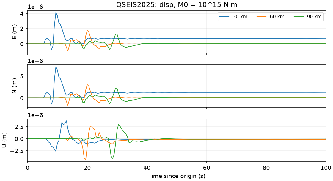
Example displacement in metres with a fixed 0–100 s horizontal axis. Time is measured from source origin because this example uses zero time reduction.

Results are under examples/output/qseis2025/. disp.npz contains the three distance traces, component labels, seconds and units; its waveform array has shape (3, 3, 201) and includes both 0 s and 100 s. summary.json records checks and run details. The solver library still contains 256 samples per trace. Use python examples/qseis2025.py --reuse to read the completed library again without launching the solver.

Add tensor outputs

Use a separate output directory so the selected quantities match the library:

python examples/qseis2025.py --observables all --output-dir examples/output/qseis2025_tensors

This enables displacement, strain and stress; it writes strain.npz/png and stress.npz/png in addition to displacement. The tensor arrays have shape (3, 6, 201) and components EE, EN, EU, NN, NU, UU. All three observables are cropped to 0–100 s inclusive before saving arrays and plots. Strain is dimensionless and stress is in Pa after the script’s explicit moment scaling.

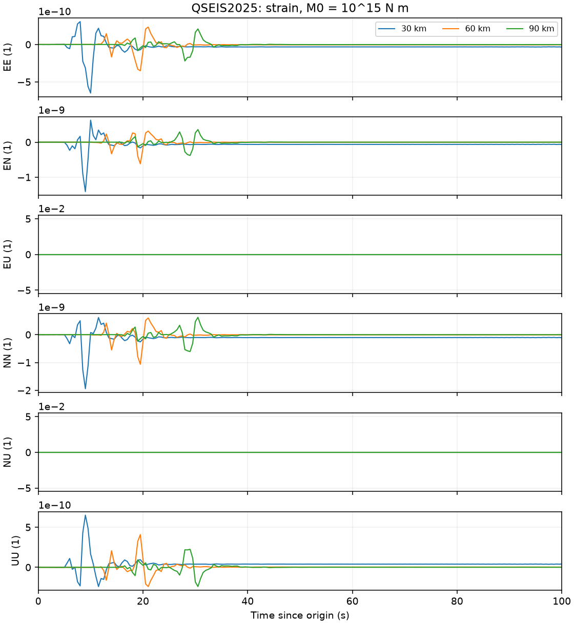
Dimensionless tensor strain at 30, 60 and 90 km, cropped to 0–100 s since source origin; shear entries are tensor strains rather than engineering shear.

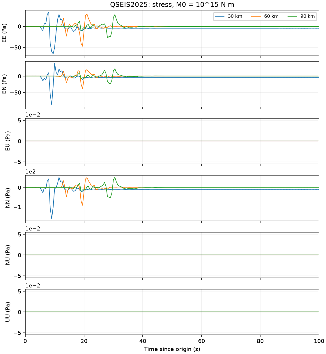
Stress in Pa for the same moment and geometry, cropped to 0–100 s since source origin. The surface receiver’s traction components can be zero under the free-surface boundary condition.

The five output_observables positions are:

Zero-based position	Family	Reader requests
0	Vector motion	disp, velo, acce
1	Fractional volume change	volume
2	Strain	strain, strain_rate
3	Stress	stress, stress_rate
4	Rotation	rota, rota_rate

Thus [1, 0, 1, 1, 0] enables the demonstrated tensor calculation. The physical stored quantity depends on wavelet_type. Here type 2 is a tapered Heaviside, so the stored non-rate kernels include displacement, strain and stress. wavelet_duration=4 means four samples, or 2 s, not four seconds.

Regional waveforms at 300, 600 and 900 km

The regional option preserves the short default tutorial and selects a separate calculation at 300, 600 and 900 km:

python examples/qseis2025.py --regional

The source remains 10 km deep and receivers remain at the surface. flat_earth_transform=True is enabled with the same 24 numeric model rows. The interval is 4 s and the native window is 4092 s, giving 1024 library samples. The saved waveforms and plots cover 0–1020 s inclusive, or 256 samples; their time zero is source origin. Results default to examples/output/qseis2025-regional/, where disp.npz has shape (3, 3, 256). The regional QSEIS, SPGRN and QSSP examples share the 4 s interval and 0.125 Hz Nyquist limit. QSEIS derives its frequency range from sampling rather than a separate max_frequency argument. The 1024-point FFT computes through 511/4096 = 0.124755859375 Hz; the Nyquist bin is zero. All regional examples use strike/dip/rake 30°/45°/90°, moment 10^15 N m and azimuth 30°.

The source uses wavelet_type=0, wavelet_duration=16 and 1024 custom moment-rate samples over 0–64 s. Its physical target is the same normalized squared half-sinusoid used by SPGRN2020 and QSSP2020. The example compensates for QSEIS’s real-frequency implementation by multiplying the input samples by exp(2*pi*fi*t), where fi<0 is the solver’s numerical-damping frequency. It does not renormalize the written samples: their area is approximately 0.9647094, whereas the effective pulse after damping correction has unit area and centroid 32 s. See the STF verification.

Custom type-0 samples are a moment-rate function, so the library stores rate kernels, as for type 1. The example requests output_type="disp" and the reader integrates velocity once using cumsum * dt over the complete native record before the script crops it. QSEIS duration is still measured in native time samples: sixteen 4 s intervals define the 64 s support, while the independent custom array has 1024 nodes. The near-distance default remains type 2 with four samples at 0.5 s.

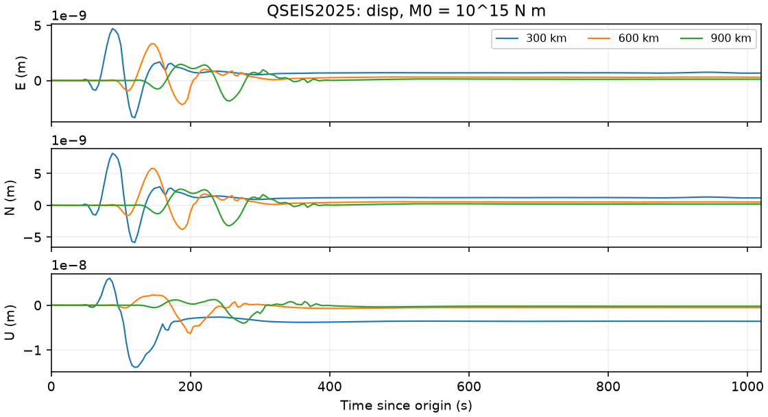
Regional displacement in metres over 0–1020 s since source origin. The calculation retains its full 4092 s native library window.

To include regional strain and stress, use:

python examples/qseis2025.py --regional --observables all --output-dir examples/output/qseis2025-regional-tensors

This additionally saves strain.npz/png and stress.npz/png, with tensor shape (3, 6, 256) and component order EE, EN, EU, NN, NU, UU. Their units and moment normalization are the same as in the near-distance tensor example. For the regional type-0 library, the script requests strain and stress directly; the reader integrates the stored strain_rate and stress_rate kernels exactly once using cumsum * dt.

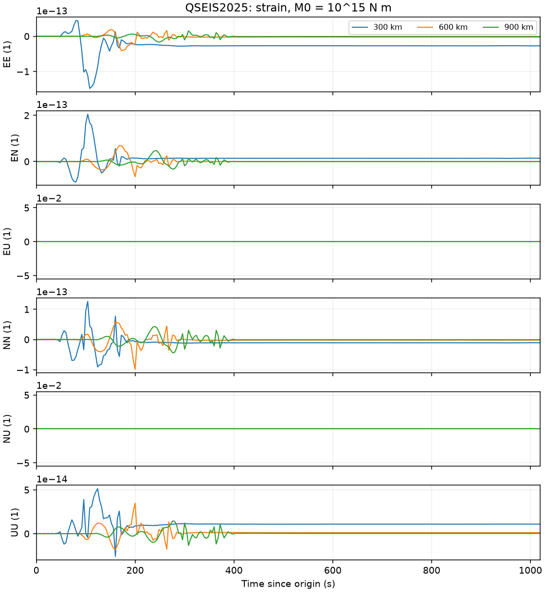
Dimensionless regional strain over 0–1020 s. Shear entries are tensor strains.

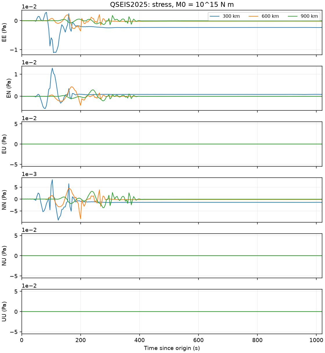
Regional stress in Pa over 0–1020 s for the same source and model.

The effective 64 s source pulse and frequency band are shared with the spherical examples. The default QSEIS2025 regional calculation retains source_radius_ratio=0.05, matching QSEIS06’s native constant. This applies frequency- and distance-dependent spatial smoothing; the spherical examples use point sources. The 24-row half-space model and its flat-Earth transformation also differ from the complete spherical model. See regional comparison limits. Reuse requires --regional and a library built with the current custom source and the same selected observables and parameters. Rebuild libraries created by the earlier type-2 regional example.

Point-source control

Run a separate regional calculation to disable the Gaussian spatial smoothing:

python examples/qseis2025.py --regional --point-source

--point-source requires --regional and sets source_radius_ratio=0. The default destination becomes examples/output/qseis2025-regional-point-source/; the standard regional library retains its 0.05 ratio. The time sampling, effective 64 s STF, mechanism, moment, model and Earth flattening remain the same. Displacement is saved as disp.npz with shape (3, 3, 256) and disp.png, together with summary.json and the source-function records.

For a positive ratio, the native solver uses

radius(f, r) = source_radius_ratio * min(sqrt(r**2 + (zs-zr)**2), Vp_source/(f+df))
multiplier(k) = exp(-(k*radius)**2/2)

Here r is epicentral distance, zs-zr is the source–receiver depth separation in the backend coordinates, Vp_source is the source-layer P-wave speed, f is frequency, df is the FFT frequency increment and k is wavenumber. Use consistent length units. The backend applies any selected Earth flattening before evaluating these quantities. The radius changes with both receiver distance and frequency; it is not a fixed-radius physical source disk. Setting the ratio to zero removes the Gaussian multiplier and also changes the automatically estimated wavenumber cutoff. This can substantially increase computation time.

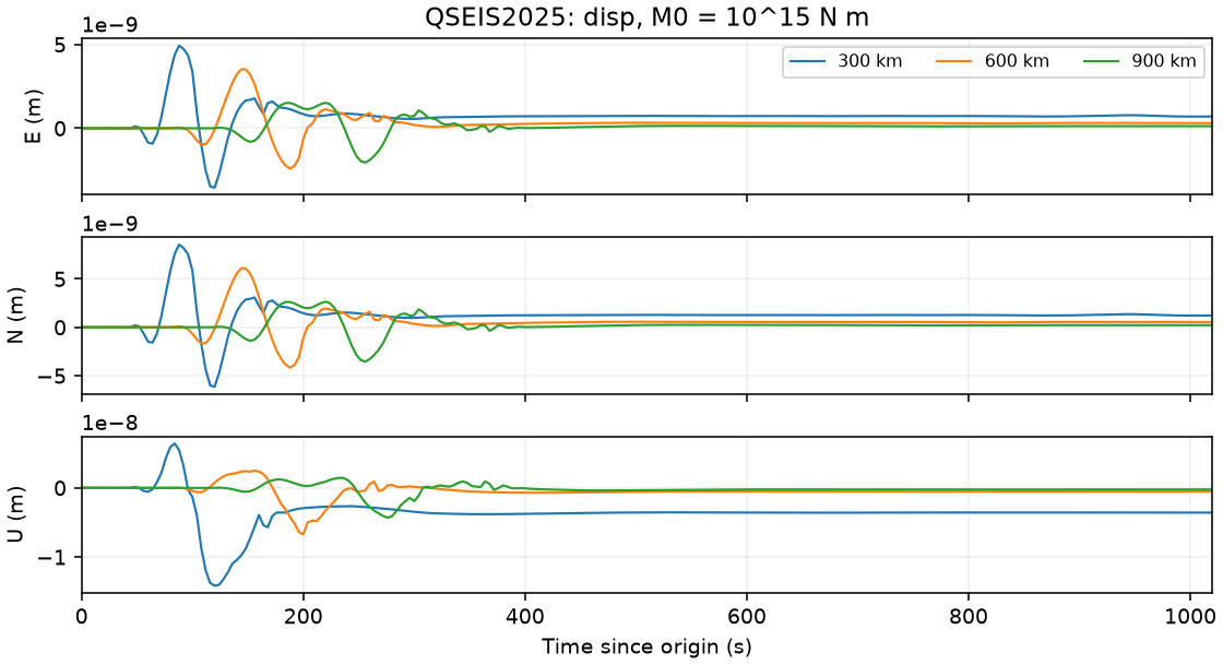
Point-source control at 300, 600 and 900 km, with the same effective 64 s STF, mechanism and 0–1020 s output window as the standard regional example.

In the archived 64 s comparison, the verified control changed only the spatial-source ratio among the numerical parameters; it requested displacement only. Relative L2 differences against the SPGRN2020 point-source calculation at 0.125 Hz were:

Distance	QSEIS2025 ratio 0.05	QSEIS2025 ratio 0
300 km	12.741%	11.493%
600 km	19.574%	17.076%
900 km	22.798%	19.718%

The comparison uses native origin-time coordinates, linearly interpolated to a common 1 s grid from each SPGRN2020 start time (3, 40 or 78 s) through 500 s. Each value is the joint ENU norm of the difference divided by the SPGRN2020 norm. No fitted amplitude scale or fitted time shift is applied.

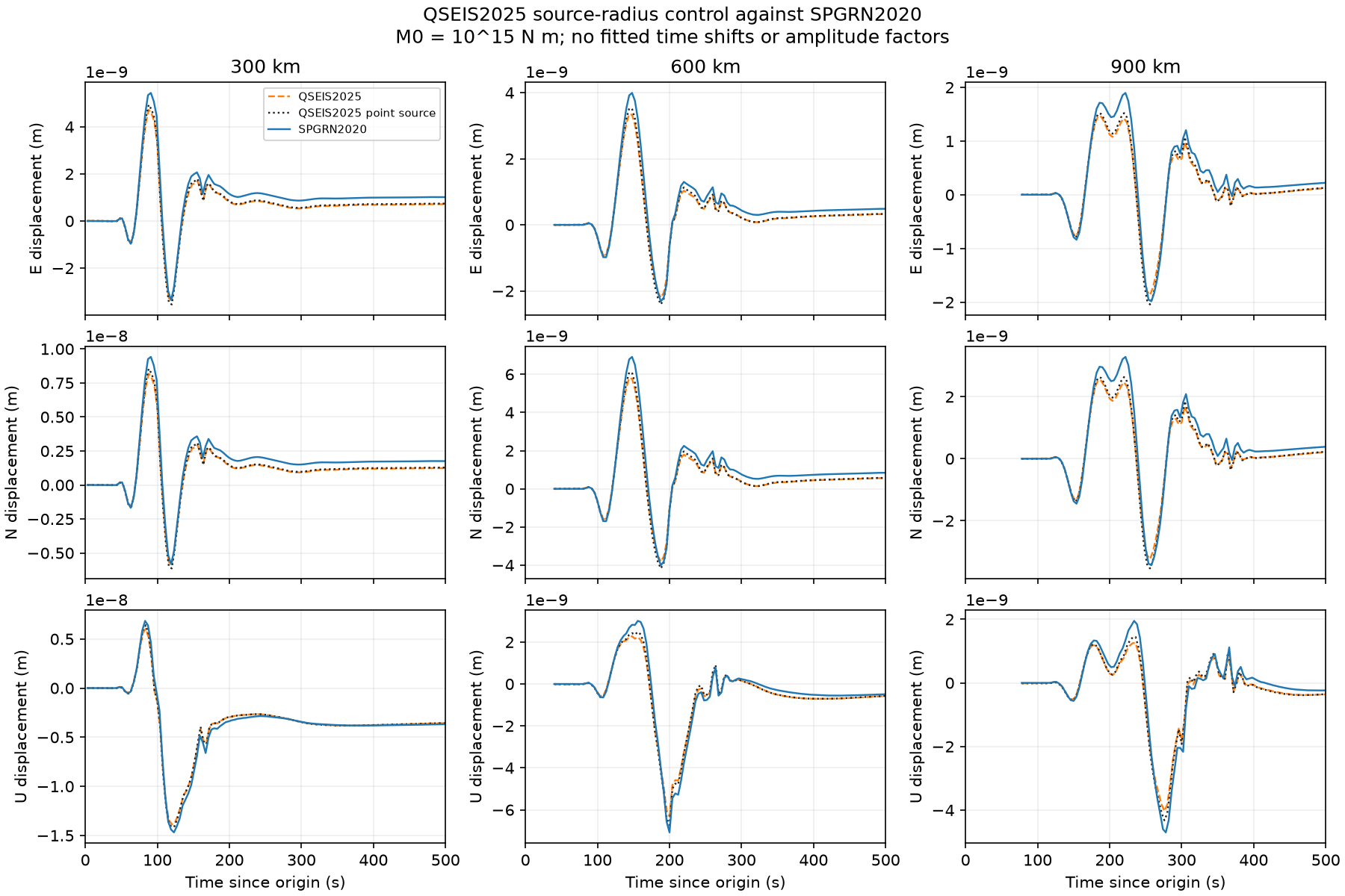
Changing the spatial-source ratio reduces part of the discrepancy. A substantial residual remains, so the control does not establish spatial smoothing as the sole cause or demonstrate convergence of all settings.

The recorded point-source run took 615.795 s on the recorded Windows environment, versus 175.929 s for the default-ratio regional run with tensors. Its arrays were finite and the native output contained no warnings or errors; runtimes depend on hardware and concurrent work. See validation for run records.

Use --regional --point-source --reuse to reread a matching point-source library. The example checks the native input’s radius ratio and wavenumber truncation tolerance as well as its other settings, and rejects a library with incompatible spatial-source controls. QSEIS06 fixes the ratio at 0.05 in its native solver; its existing Python API has no equivalent flag.

Parameters that control the calculation

N_each_group splits receiver distances into jobs; it is 3 in this example. It controls job size and file layout, not the source model. wavenumber_sampling_rate, anti_alias, slowness_int_algorithm and an optional slowness_window control integration. QSEIS2025 additionally exposes eps_estimate_wavenumber and source_radius_ratio. Establish convergence when changing band, distance or depth.

time_reduction_velo is km/s; zero means no reduction. The raw free_surface switch is the backend partial-solution switch, with 0 retaining free-surface effects. It is not the same Python boolean interface as QSEIS06’s free_surface.

The reader supports nearest or trilinear interpolation, ENZ rotation, optional arrival adjustments and filtering/resampling. See reading. An output family’s source files must exist before its derived rate/non-rate version can be requested.

Outputs and limitations

Each depth pair contains distance-group directories with grn.inp and basis files prefixed ex, ss, ds and cl. Components e* are strain and s* are stress, despite swapped labels in some template comments. The example retains ASCII and creates reader-compatible binary files. Keep green_lib_info.json and travel-time tables with the data.

At rotate=False, six-component tensor output is a north-reference ENZ basis, not the vector’s RTZ convention. Use rotate=True and the documented component order for comparison.

The tutorial verifies executable output and reader behavior. A 30 km distance grid and its integration defaults do not validate interpolation, high frequencies, zero-distance behavior or interface stresses for your study.