Earlier comparison with a 64 s source

This archived report documents the 0.125 Hz Nyquist band, 64 s STF, 4 s sampling and surface receiver used by the lightweight regional examples. References to “current” results below refer to this configuration. These measurements remain valid for those recorded runs.

The latest comparison uses fresh AK135-FC libraries, a 2 Hz Nyquist band, a 1.25 s STF and a receiver at 1 km depth. It includes six-component stress and an isolated QSEIS06 point-source control. The standard regional tutorial commands below reproduce this earlier protocol.

This report compares QSEIS06, QSEIS2025, SPGRN2012, SPGRN2020 and QSSP2020 with a common temporal frequency band, mechanism and effective 64 s moment-rate pulse. These matched conditions do not make the numerical models identical. The earlier unequal-band calculation and harmonic parameter scans remain in the historical report.

After matching the effective STF

SPGRN2020 with max_slowness=0 is the numerical reference, not an absolute reference solution. The relative L2 metric is

\[ 100\,\frac{\lVert u-u_{\rm ref}\rVert_2}{\lVert u_{\rm ref}\rVert_2}, \]

over east, north and up displacement together. Each distance uses linear interpolation onto a 1 s grid through 500 s, starting at the latest native start among the five backends: 3, 40 and 78 s respectively. No fitted time shift, amplitude scale or baseline removal is applied.

Calculation versus SPGRN2020	300 km	600 km	900 km
QSEIS06, default spatial source	12.7410%	19.5740%	22.7979%
QSEIS2025, default spatial source	12.7410%	19.5740%	22.7979%
SPGRN2012, matched effective STF	1.2266%	0.0739%	0.0535%
QSSP2020, harmonic controls 2000/8000	1.2772%	0.4085%	2.3022%

The default QSEIS versions produced exactly equal saved displacement samples in this run. The script retains two checks: the QSEIS version pair over all saved samples (rtol=1e-5, atol=1e-20 m), and QSSP2020 versus SPGRN2020 below 5% at each distance. Both pass; the checks do not assert agreement of every backend pair.

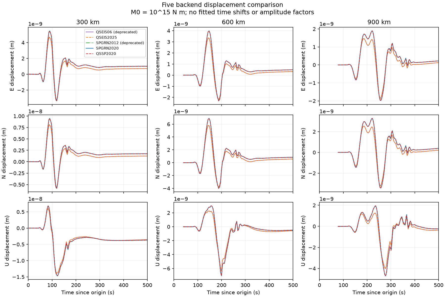
Current comparison on physical source-origin time axes. The default QSEIS pair still has substantial differences from SPGRN2020.

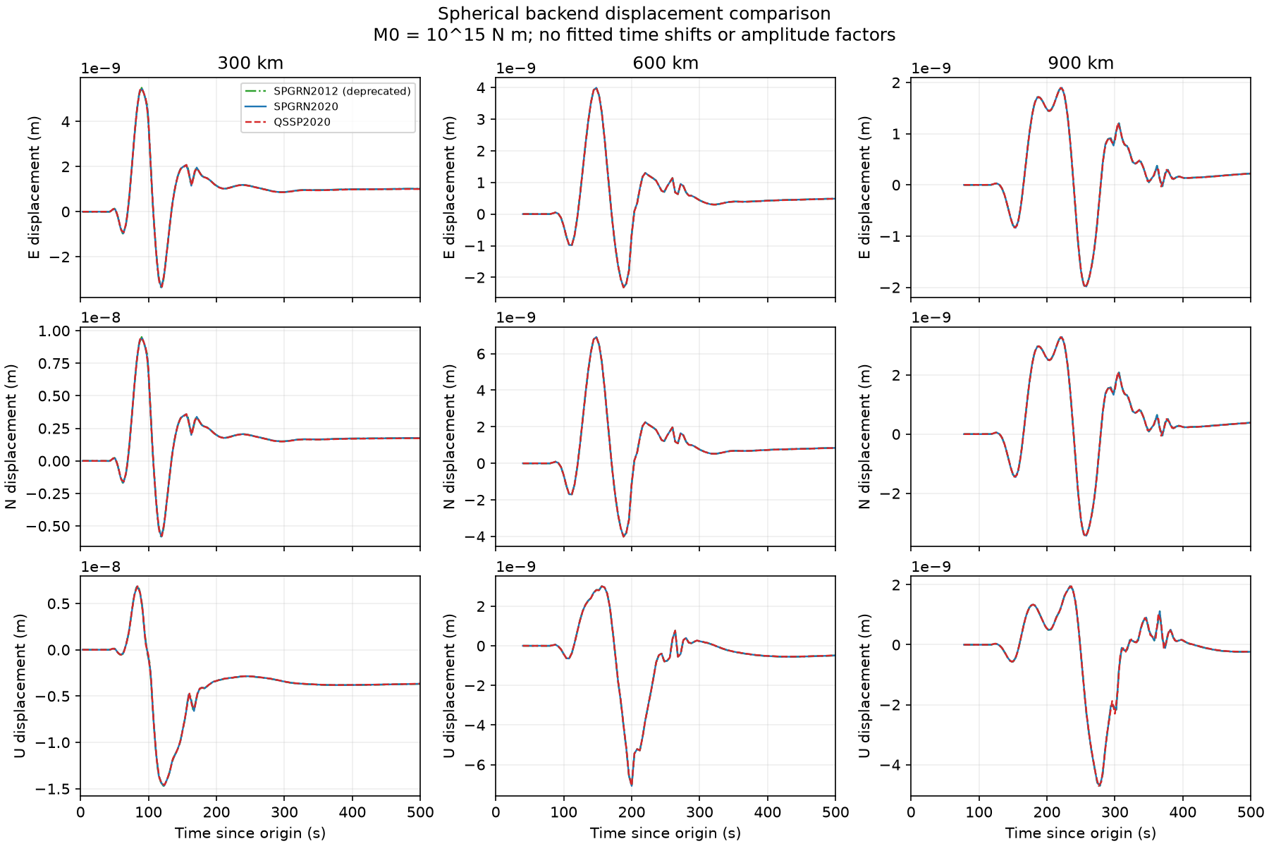
Spherical examples with the effective 64 s pulse and common Nyquist band.

Download the current comparison record for component metrics, input hashes, source evidence and native spectral settings.

Common physical and frequency settings

The examples use the bundled AK135 elastic profile with illustrative constant Qp=600 and Qs=300, rather than the original AK135-F attenuation. Source depth is 10 km, receiver depth is zero, distances are 300/600/900 km, and receiver azimuth is 30°. The shared strike/dip/rake is 30°/45°/90°, scalar moment is 1e15 N m, and displacement is ENU in metres. The spherical examples enable spheroidal and toroidal motion, with self-gravitation and physical dispersion disabled.

Temporal setting	All five regional calculations
Native sampling interval	4 s
FFT sample count N	1024
Requested spectral/native QSEIS span	4092 s
FFT period N dt	4096 s
Frequency spacing df	1/4096 = 0.000244140625 Hz
Requested upper frequency / Nyquist	0.125 Hz
Retained nonnegative bins	512, including zero frequency
Highest computed frequency	511/4096 = 0.124755859375 Hz
Nyquist bin at 0.125 Hz	Set to zero
Anti-aliasing factor	0.01
Exported displacement shape	(3 distances, 3 components, 256 samples)

QSEIS derives its frequency range from the time grid. The spherical inputs explicitly request max_frequency=0.125. Their native routines use nfcut=min(nf, 1+nint(fcut/df)), retaining bins zero through 511 and zeroing the separate Nyquist endpoint. The 64 s pulse is not strictly band-limited; this solver cutoff is distinct from a source corner frequency.

The actual damping conventions are:

Solver	Imaginary frequency fi
QSEIS06/2025	ln(0.01)/(2*pi*4092) = -0.000179114271475911 Hz
SPGRN2012/2020 and QSSP2020	ln(0.01)/(2*pi*4096) = -0.000178939355195173 Hz

The source construction uses these respective damping frequencies, even though the real-frequency grids agree.

Matching the effective source time function

The common physical moment-rate pulse is

\[ r(t)=\frac{2}{T}\sin^2\left(\frac{\pi t}{T}\right), \qquad 0\leq t\leq T,\quad T=64\ {\rm s}, \]

and zero elsewhere. Its integral is one and its centroid is 32 s. The shared REGIONAL_STF in examples/common.py is recorded as physical_source_time_function in every summary.

SPGRN2020 and QSSP2020 evaluate this pulse at complex frequency. QSEIS uses wavelet_type=0 with 1024 source nodes over 0–64 s, separate from the 4 s seismogram grid. Written node values are r(t_j) exp(2*pi*fi*t_j); do not renormalize these compensated inputs. Fortran’s final damping correction restores the physical pulse from their piecewise-linear interpolant. Its archived time-domain relative L2 error is 1.988e-6 and spectral relative L2 error over 0–0.125 Hz is 1.783e-6. Effective area is approximately 1.000000000413 and centroid 32.000000734 s, within the recorded tolerances.

SPGRN2012 now uses source_duration=0, selecting its native unit-spectrum impulse branch. It exports the complete 1024-sample, 4092 s velocity span with max_slowness=0. The example restores damping, transforms each full Green-function record, multiplies by the analytic transform of r(t) at f+i*fi, inverts, and removes damping. This is forward convolution, with no deconvolution or fitted scaling. Only then does the reader, called with output_type="disp" on the source-matched library, integrate once using cumsum * dt; the example exports 256 displacement samples. The summary distinguishes the native zero duration from the effective physical duration of 64 s.

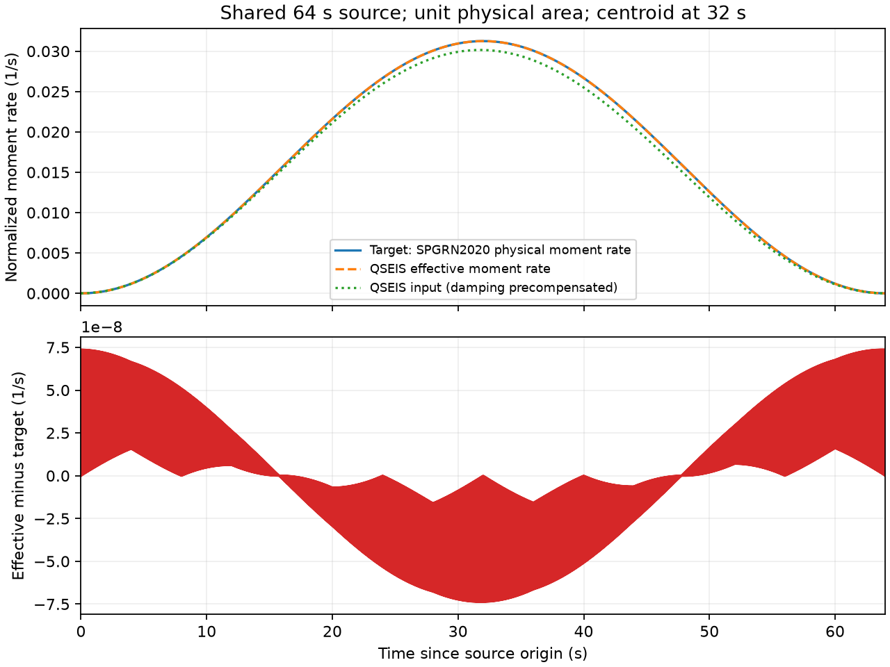
The normalized 64 s physical pulse and its numerical verification.

The helpers source_time_function.py and spherical_source_time_function.py archive definitions, source samples or transfer functions, and file hashes. The source verification preserves the QSEIS checks. SPGRN2012 also saves its source-matched Green-function library and analytic transfer function.

QSEIS at the same regional distances

The default QSEIS pair retains the same Gaussian spatial smoothing. In the wavenumber integral, the kernel is multiplied by

\[ G(k,f,d)=\exp\left[-\frac{1}{2}\{k\,a(f,d)\}^2\right], \qquad a(f,d)=\rho\,\min\left[ \sqrt{d^2+(z_s-z_r)^2},\, \frac{v_{P,s}}{f+df} \right]. \]

Here k is horizontal wavenumber; d, the depths and source-layer P velocity are the solver’s working coordinates and model values. The dimensionless rho is source_radius_ratio. This frequency- and distance-dependent spatial smoothing is separate from the temporal STF. See the multiplication in QSEIS2025 qswvint.f.

QSEIS06 fixes rho=0.05 inside Fortran. QSEIS2025 exposes the parameter; its default regional run also uses 0.05 to preserve the version-pair comparison. The spherical examples set source_radius=0.

Optional point-source control

QSEIS2025 --regional --point-source sets rho=0, making G=1. The remaining requested model, temporal source and frequency settings stay the same. Radius also enters automatic wavenumber-limit estimation, so the control changes that numerical setting as implemented by the solver.

QSEIS2025 versus SPGRN2020	300 km	600 km	900 km
Default rho=0.05	12.7410%	19.5740%	22.7979%
Point-source control rho=0	11.4926%	17.0758%	19.7176%

This reduces the relative differences by about 1.25–3.08 percentage points, leaving an 11–20% residual. It does not establish that spatial smoothing explains the dominant discrepancy or isolate the remaining contributions. The control has no additional pass/fail threshold.

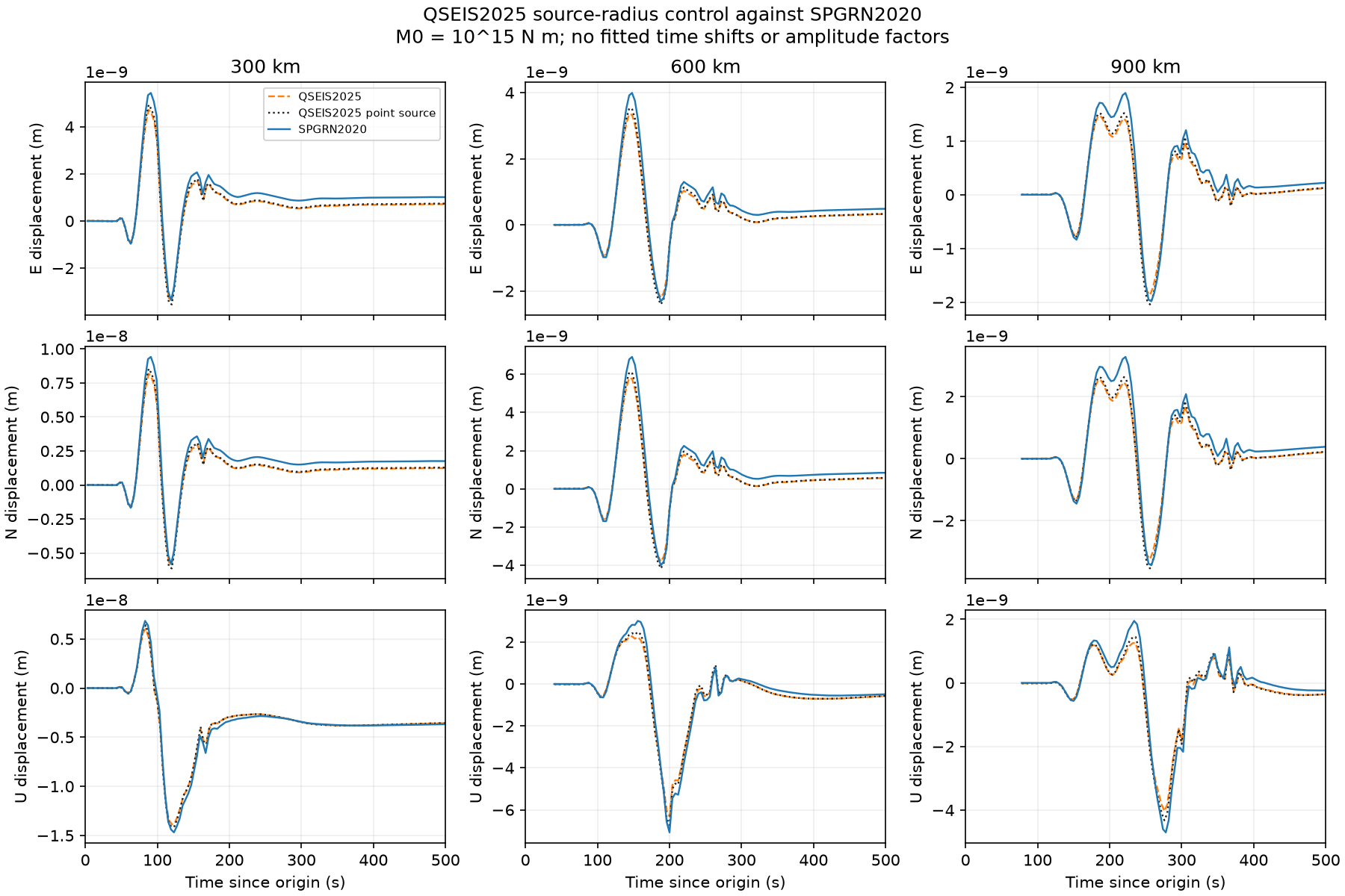
Effect of the QSEIS2025 radius setting on the same comparison grids.

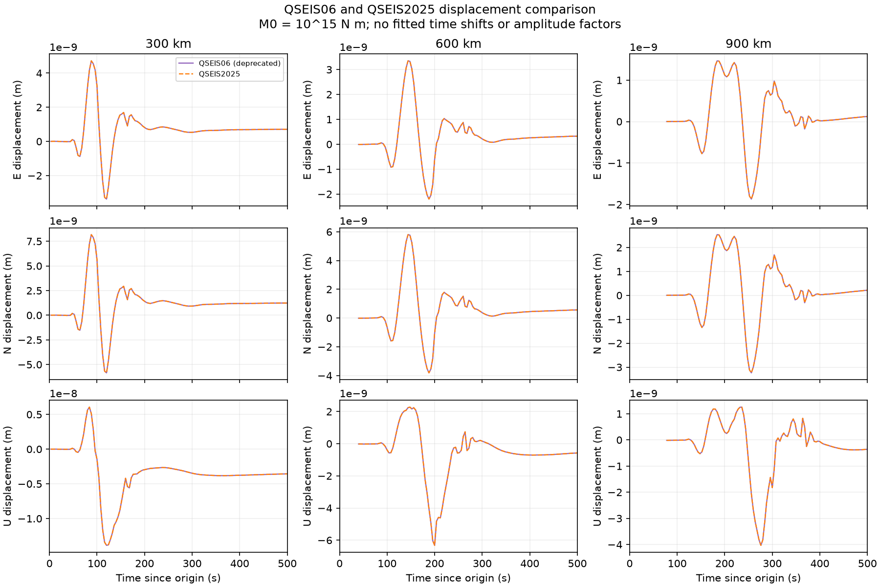
The standard version pair retains its common radius ratio of 0.05.

Time origins, model boundaries and spatial convergence

Native starts, in seconds since source origin, are:

Backend	300 km	600 km	900 km
QSEIS06/2025 and QSSP2020	0	0	0
SPGRN2012	-10	20	50
SPGRN2020	3	40	78

SPGRN2012 rounds t0 + distance/v0; SPGRN2020 rounds the P onset minus green_before_p. The examples read those native start records. Compare physical times, not sample indices, without fitting a 32 s source-centroid shift. The 256 exported samples span 1020 s from each start.

QSEIS uses a 24-row layered model continued as a half-space, with the flat-Earth transformation enabled; the spherical examples use the complete Earth profile. Flattening does not restore omitted deep structure. Integration also differs: the Python readers use cumsum * dt, while QSSP accumulates displacement in Fortran from a zero initial value. Model boundaries, spatial truncation and integration baselines remain distinct; their individual contributions have not been isolated.

Spherical setting	Actual maximum degree in the new native spectrum header
SPGRN2012, max_slowness=0	5293
SPGRN2020, max_slowness=0	4304
QSSP2020, min_harmonic=2000, max_harmonic=8000	2001

A zero slowness input selects automatic full-wavefield truncation in SPGRN; the sum remains finite. QSSP’s minimum constrains its frequency-dependent upper cutoff; it does not exclude low degrees. Its maximum also affects allocation and spatial differential filtering in synthesis. Equal spectrum files therefore need not give equal waveforms after changing that maximum.

These header values are observations, not general convergence guarantees. The historical parameter sweep used 0.0625 Hz and does not establish convergence at 0.125 Hz. Further checks must vary spatial controls, model extent and integration/window choices separately.

Reproduce and verify

From a clean checkout, run the five examples and compare their saved arrays:

python examples/qseis06.py --regional
python examples/qseis2025.py --regional
python examples/spgrn2012.py
python examples/spgrn2020.py
python examples/qssp2020.py
python examples/compare_backends.py

Add the separately reported radius control with:

python examples/qseis2025.py --regional --point-source
python examples/compare_backends.py --qseis2025-point-source examples/output/qseis2025-regional-point-source

On Windows with Conda, prefix Python commands with conda run -n YOUR_ENV. Use fresh --output-dir directories when outputs already exist. Comparison backend options accept an example directory or its disp.npz. An old library cannot gain the new frequency band or STF through --reuse or an edited summary.

Every current summary includes spectral_settings. spectral_settings.py reads spherical native headers and verifies nt=ntcut=1024, dt=4, nf=nfcut=512, df=1/4096. For QSEIS it verifies native input and all output time labels, then derives nf and df using the solver’s formula: the text header does not store them. The report identifies the evidence source and records fi and the actual harmonic cutoff.

compare_backends.py repeats these checks against the libraries and summaries, validates archived effective sources, and rejects an old 0.0625 Hz band or inconsistent STF. The optional control also checks QSEIS2025’s native radius input. Three standard comparison figures and comparison.json are written; source-radius-comparison.png and control metrics are added only when control data are supplied. Preserve native inputs, source evidence and models alongside the arrays to keep these checks repeatable.