QSEIS06 (deprecated): vector waveforms#

Deprecated

The QSEIS06 backend is deprecated in pygrnwang. Use QSEIS2025 for new calculations. This tutorial and its interfaces remain available for existing workflows. Migration requires building a QSEIS2025 library and validating the numerical settings, source time function and output conventions.

QSEIS06 provides the established layered half-space vector workflow. The main reader returns displacement, velocity or acceleration. It remains useful for reproducing QSEIS06 calculations and comparing an established library with the newer direct-observable workflow.

The fresh comparison dated 2026-09-15 uses 0.25 s sampling, a 2 Hz Nyquist limit, a 1.25 s effective source pulse and receivers 1 km deep at 300, 600 and 900 km. It is separate from the near-distance and 64 s regional tutorials below; these commands do not produce the new comparison figures.

That comparison retains stock QSEIS06’s frequency-dependent Gaussian smoothing and adds an isolated rd2r=0 point-source control build. The control is not the released backend or an option in its Python API. For the tested settings, stock QSEIS06 and ratio-0.05 QSEIS2025 have bit-identical saved displacement arrays, as do the two point-source controls. See the comparison for the limits of this result.

Complete calculation#

python examples/qseis06.py

The default near-distance mode builds one 10 km source depth and a surface receiver at 30, 60 and 90 km, using a 0.5 s interval and 127.5 s window. Like the default QSEIS2025 example, it uses 24 numeric model rows and no flat-Earth transformation. The source has strike/dip/rake 30°/45°/90° and moment 10^15 N m.

Complete QSEIS06 tutorial#

"""Deprecated QSEIS06 tutorial; use qseis2025.py for new calculations.

Retained to build, read and plot existing QSEIS06 workflows. Migration requires
rebuilding the library and validating the replacement backend settings.
"""
from pathlib import Path

from common import (MECHANISM, MOMENT_NM, REGIONAL_SAMPLING_INTERVAL_S, REGIONAL_STF, finish, parser_for, prepare,
                    require_library_settings, save_waveforms)
from pygrnwang.create_qseis06_bulk import (
    pre_process_qseis06, create_grnlib_qseis06_sequential)
from pygrnwang.read_qseis06 import seek_qseis06
from source_time_function import prepare_qseis_stf, validate_qseis_stf
from spectral_settings import qseis_spectral_settings


def main():
    parser = parser_for("qseis06")
    parser.add_argument("--regional", action="store_true",
                        help="Use 300/600/900 km, a 64 s wavelet and Earth flattening")
    parser.set_defaults(output_dir=None)
    args = parser.parse_args()
    if args.output_dir is None:
        directory = "qseis06-regional" if args.regional else "qseis06"
        args.output_dir = Path(__file__).resolve().parent / "output" / directory
    output, library, model, report, started = prepare(
        args, "QSEIS06", extra={"display_name": "QSEIS06 (deprecated)"})
    dt, window = (REGIONAL_SAMPLING_INTERVAL_S, 4092.0) if args.regional else (0.5, 127.5)
    distances = [300.0, 600.0, 900.0] if args.regional else [30.0, 60.0, 90.0]
    wavelet_duration = 16 if args.regional else 4
    wavelet_type = 0 if args.regional else 2
    source_time_function = None
    output_end = 1020.0 if args.regional else window
    output_samples = int(round(output_end / dt)) + 1
    native_samples = int(round(window / dt)) + 1
    if not args.reuse:
        pre_process_qseis06(
            processes_num=1, path_green=library, event_depth_list=[10.0],
            receiver_depth_list=[0.0], dist_range=[distances[0], distances[-1]],
            delta_dist=distances[0],
            N_each_group=3, time_window=window, sampling_interval=dt,
            wavelet_type=wavelet_type, wavelet_duration=wavelet_duration, time_reduction_velo=0,
            flat_earth_transform=args.regional, path_nd=model, earth_model_layer_num=24,
        )
        if args.regional:
            source_time_function = prepare_qseis_stf(
                library, duration_s=64.0, samples=1024)
        create_grnlib_qseis06_sequential(library, remove_pd=False)
    require_library_settings(
        library, event_depth_list=[10.0], receiver_depth_list=[0.0],
        grn_dist_range=[distances[0], distances[-1]], grn_delta_dist=distances[0],
        sampling_interval=dt, time_window=window, sampling_num=native_samples,
        wavelet_type=wavelet_type, wavelet_duration=wavelet_duration, time_reduction_velo=0,
        flat_earth_transform=args.regional, earth_model_layer_num=24,
        slowness_window=None, wavenumber_sampling_rate=12, anti_alias=0.01,
        free_surface=True,
    )
    if args.regional and args.reuse:
        source_time_function = validate_qseis_stf(library)
    # Regional type-0 kernels are rates; the reader integrates them before cropping.
    arrays = [MOMENT_NM * seek_qseis06(
        path_green=library, event_depth_km=10.0, receiver_depth_km=0.0,
        az_deg=30.0, dist_km=distance, focal_mechanism=MECHANISM,
        srate=1 / dt, output_type="disp", rotate=True,
        before_p=None, shift=False, pad_zeros=False,
    )[:, :output_samples] for distance in distances]
    save_waveforms(output, report, "disp", arrays, distances, dt, ["E", "N", "U"], "m",
                   expected_samples=output_samples,
                   time_limits=(0.0, output_end) if args.regional else None)
    report.update(sampling_interval_s=dt, max_frequency_hz=0.5 / dt, time_window_s=window, distances_km=distances,
                  output_time_range_s=[0.0, output_end], native_samples=native_samples,
                  earth_model_numeric_rows=24, wavelet_type=wavelet_type,
                  wavelet_duration_samples=wavelet_duration,
                  wavelet_duration_s=wavelet_duration * dt,
                  flat_earth_transform=args.regional, regional=args.regional, source_radius_ratio=0.05)
    if args.regional:
        report["source_time_function"] = source_time_function
        report["physical_source_time_function"] = dict(REGIONAL_STF)
        report["spectral_settings"] = qseis_spectral_settings(library)
    finish(output, report, started)


if __name__ == "__main__":
    main()

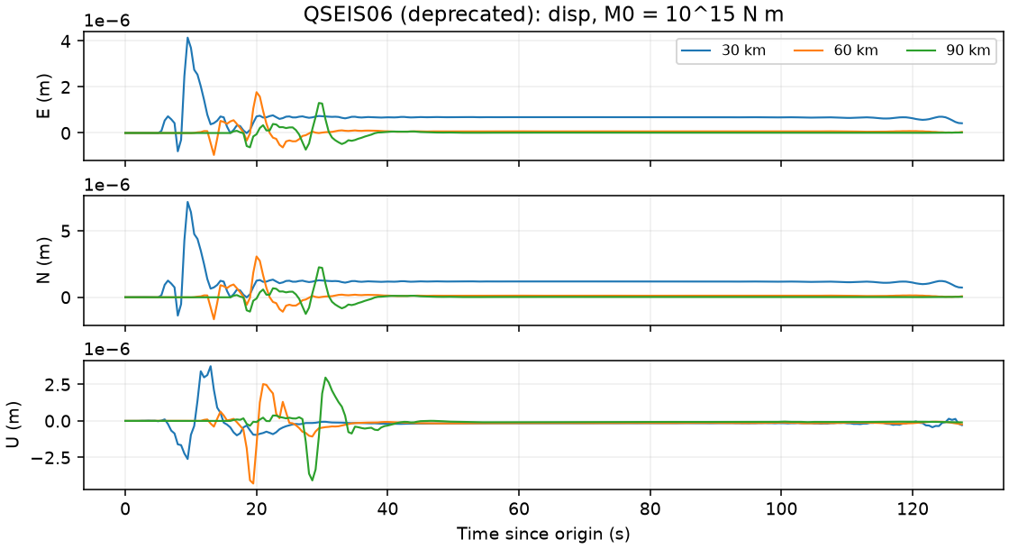
QSEIS06 east, north and up displacement for three distances. — Displacement in metres, plotted against seconds since source origin.#

Expect disp.npz with waveform shape (3, 3, 256), disp.png, summary.json and a library beneath examples/output/qseis06/. --reuse rereads that library.

Regional waveforms at 300, 600 and 900 km#

Run the same script with the regional option:

python examples/qseis06.py --regional

This selects 300, 600 and 900 km while retaining a 10 km source and surface receiver. It enables flat_earth_transform=True and keeps the same 24 numeric model rows. A 4 s interval and 4092 s native window give 1024 library samples. After synthesis, the script saves 0–1020 s inclusive, or 256 samples, under examples/output/qseis06-regional/. The resulting disp.npz has shape (3, 3, 256) and a source-origin time axis. The regional QSEIS, SPGRN and QSSP examples share the 4 s interval and 0.125 Hz Nyquist limit. QSEIS obtains its frequency range from the sampling interval rather than a separate max_frequency argument. With 1024 FFT samples, the final computed positive-frequency bin is 511/4096 = 0.124755859375 Hz; the Nyquist bin is zero.

The regional source uses wavelet_type=0, wavelet_duration=16 with 1024 custom moment-rate samples spanning 0–64 s. The physical target is a normalized squared half-sinusoid. Before writing the input, the example multiplies its samples by exp(2*pi*fi*t) to compensate for QSEIS’s numerical damping convention; fi is negative. The written samples are not renormalized: their area is approximately 0.9647094, while the effective physical pulse has unit area and a 32 s centroid. The STF verification checks the actual pulse and its spectrum against the target.

A custom type-0 pulse is a moment-rate function, so the library stores velocity kernels, as for type 1. This example requests output_type="disp"; the reader integrates once using cumsum * dt over the complete native record, and the script then crops and saves displacement. The default near-distance example retains type 2 with four 0.5 s samples; its behavior is unchanged.

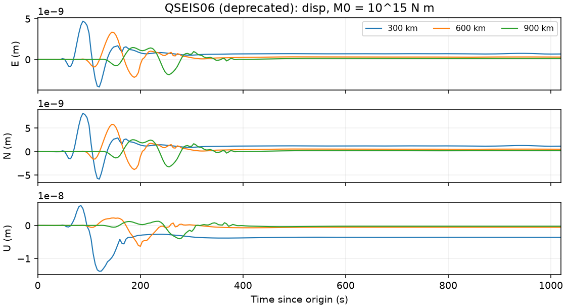
QSEIS06 regional displacement at 300, 600 and 900 km. — Regional displacement in metres, saved from 0 to 1020 s since source origin. The native 4092 s library window is retained.#

The regional examples share the effective 64 s moment-rate pulse, strike/dip/rake 30°/45°/90°, moment 10^15 N m and azimuth 30°. Matching those settings and the frequency band does not make the half-space and spherical calculations identical.

QSEIS06 also applies frequency- and distance-dependent Gaussian spatial smoothing. The native solver fixes its radius ratio at 0.05; the current Python API cannot turn it off. The radius at each receiver and frequency is 0.05 times the smaller of the source–receiver separation and Vp_source/(f + df), using the backend’s model coordinates and source-layer P-wave speed. Its wavenumber multiplier is exp(-(k*radius)**2/2). This differs from the spherical examples’ point sources even when their effective time functions agree. The default QSEIS2025 regional example retains the same 0.05 ratio for comparison with QSEIS06.

In the archived 64 s comparison, the QSEIS2025 point-source control turns off this spatial smoothing. It reduces the discrepancy against SPGRN2020, but the measured relative differences remain 11.493%, 17.076% and 19.718% at 300, 600 and 900 km. Spatial smoothing therefore explains only part of the discrepancy. See the regional comparison limits for the remaining differences in geometry, model and numerical treatment.

Use --regional --reuse only for a completed library with the current custom source and matching regional parameters. A library from the earlier type-2 regional example must be rebuilt.

Source, sampling and boundary parameters#

wavelet_type=2 selects the tapered Heaviside. In the default near-distance mode, wavelet_duration=4 is four samples (2 s). Type 1 instead stores a velocity-like kernel; the reader integrates/differentiates as required. output_type is disp, velo or acce.

time_reduction_velo is km/s and zero disables reduction. free_surface=True retains free-surface effects; the writer translates this boolean into the backend switch. flat_earth_transform controls the geometric transformation; preserve it when reproducing a library.

N_each_group is the number of receiver distances per backend job. wavenumber_sampling_rate, slowness_int_algorithm, slowness_window and anti_alias affect integration and must be checked for convergence. The ordinary reader chooses nearest source depth, receiver depth and distance; it does not provide interpolate_type.

Separate finite-difference tensor workflow#

pre_process_qseis06_strain_rate creates extra distance/depth samples for the derivative readers. Its stencil uses diff_accu_order, radial increment ratio k_dr and depth increment dz in km. An ordinary vector library does not contain those additional samples.

seek_qseis06_strain_rate_diff and seek_qseis06_stress_rate_diff are separate advanced interfaces. The latter uses elastic moduli for tensor conversion. They require stencil convergence, layer/interface treatment and rotation checks appropriate to the intended calculation. Keep derivative ASCII outputs with convert_pd2bin=False, remove_pd=False because the current derivative binary detection/call path is inconsistent; see known limitations. The QSEIS2025 tensor example is the tested introductory route to direct strain and stress.

Stored data and interpretation#

A source/receiver directory contains distance groups and basis response files. Normal vector groups end in _0; derivative libraries can have additional offset groups. The tutorial keeps ASCII while preparing the binary representation for the reader. Retain metadata and matching travel-time tables.

rotate=True returns E/N/up vectors. only_seismograms=False includes nearest grid metadata; new first_p/first_s are still None unless shift=True. Numerical agreement with another backend requires consistent model, source wavelet, amplitude and time reference.