QSSP2020: spectra followed by synthetic waveforms#

QSSP2020 calculates spherical-Earth responses with optional self-gravitation and vector, tensor, rotation and gravity observables. A fresh library requires a spectral calculation before time-domain synthesis.

The fresh comparison dated 2026-09-15 includes five-backend displacement and a QSSP2020/QSEIS2025 six-component stress comparison, with 0.25 s sampling, a 2 Hz Nyquist limit, a 1.25 s effective source pulse and receivers 1 km deep. Its spectra, harmonic settings and rate integration were prepared separately. The displacement-only tutorial below retains 4 s sampling, a 64 s source and surface receivers; it does not produce those new waveforms or stress figures.

Complete displacement calculation#

python examples/qssp2020.py

The script first preprocesses spectral and six moment-source tasks, then calls the sequential builder with cal_spec=True. Time-domain synthesis consumes the resulting spectra.

Complete QSSP2020 tutorial with the spectral stage enabled#

"""Build QSSP2020 spectra first, then synthesize a small displacement library."""
from common import (MECHANISM, MOMENT_NM, REGIONAL_SAMPLING_INTERVAL_S, REGIONAL_MAX_FREQUENCY_HZ, REGIONAL_SOURCE_DURATION_S, REGIONAL_STF, finish, parser_for, prepare,
                    require_library_settings, save_waveforms)
from pygrnwang.create_qssp2020_bulk import (
    pre_process_qssp2020, create_grnlib_qssp2020_sequential)
from pygrnwang.read_qssp2020 import seek_qssp2020
from spectral_settings import verify_spherical_spectrum


def main():
    args = parser_for("qssp2020").parse_args()
    output, library, model, report, started = prepare(args, "QSSP2020")
    dt, window = REGIONAL_SAMPLING_INTERVAL_S, 1020.0
    distances = [300.0, 600.0, 900.0]
    if not args.reuse:
        pre_process_qssp2020(
            processes_num=1, path_green=library, event_depth_list=[10.0],
            receiver_depth_list=[0.0], spec_time_window=4092.0,
            sampling_interval=dt, max_frequency=REGIONAL_MAX_FREQUENCY_HZ, max_slowness=0.3,
            anti_alias=0.01, turning_point_filter=0, turning_point_d1=0.0,
            turning_point_d2=6371.0, free_surface_filter=1,
            gravity_fc=0.0, gravity_harmonic=0, cal_sph=1, cal_tor=1,
            min_harmonic=2000, max_harmonic=8000, source_radius=0.0,
            source_duration=REGIONAL_SOURCE_DURATION_S, output_observables=[1] + [0] * 10,
            time_window=window, time_reduction=0.0,
            dist_range=[300.0, 900.0], delta_dist=300.0,
            path_nd=model, earth_model_layer_num=None, physical_dispersion=0,
        )
        # Required for a fresh library: time-domain synthesis consumes GreenSpec.
        create_grnlib_qssp2020_sequential(library, cal_spec=True, remove_pd=False)
    require_library_settings(library, min_harmonic=2000, max_harmonic=8000,
                             sampling_interval=dt, time_window=window, max_frequency=REGIONAL_MAX_FREQUENCY_HZ, spec_time_window=4092.0,
                             source_duration=REGIONAL_SOURCE_DURATION_S, max_slowness=0.3,
                             grn_dist_range=[300.0, 900.0], grn_delta_dist=300.0)
    arrays = [MOMENT_NM * seek_qssp2020(
        path_green=library, event_depth_km=10.0, receiver_depth_km=0.0,
        az_deg=30.0, dist_km=distance, focal_mechanism=MECHANISM,
        srate=1 / dt, output_type="disp", rotate=True,
        before_p=None, shift=False, pad_zeros=False,
    ) for distance in distances]
    save_waveforms(output, report, "disp", arrays, distances, dt, ["E", "N", "U"], "m")
    report.update(sampling_interval_s=dt, time_window_s=window, distances_km=distances,
                  spec_time_window_s=4092.0, max_frequency_hz=REGIONAL_MAX_FREQUENCY_HZ, harmonic_bounds=[2000, 8000], source_duration_s=REGIONAL_SOURCE_DURATION_S)
    report["physical_source_time_function"] = dict(REGIONAL_STF)
    report["spectral_settings"] = verify_spherical_spectrum(library, "qssp2020")
    report["source_radius_km"] = 0.0
    finish(output, report, started)


if __name__ == "__main__":
    main()

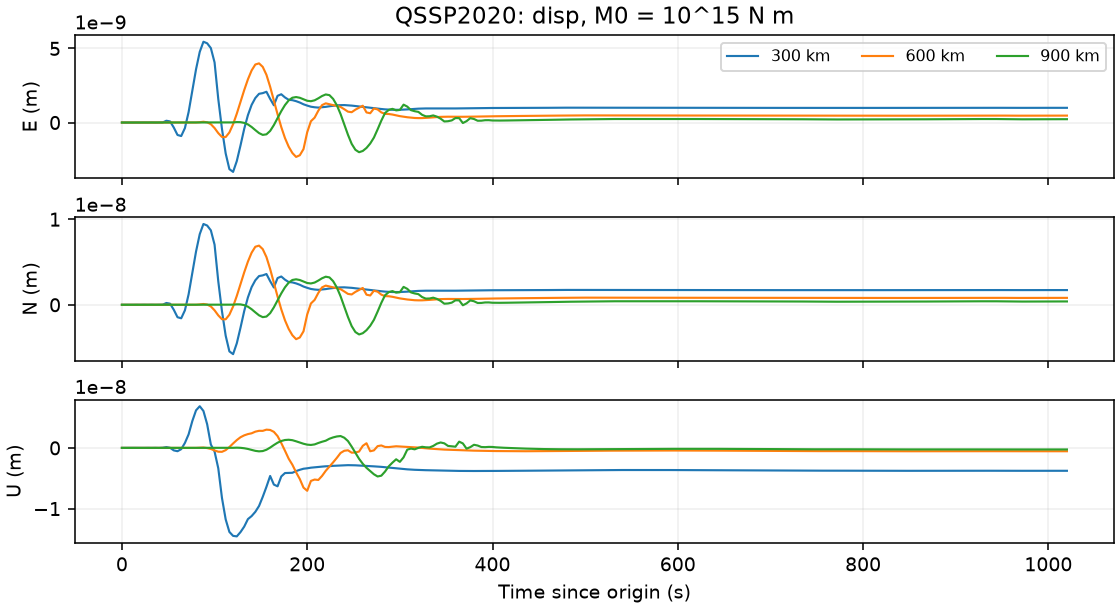
QSSP2020 east, north and up displacement at three distances. — Displacement in metres. This example uses zero time reduction, so the horizontal axis is seconds since source origin.#

The model spans the full Earth. A 10 km source and surface receiver are sampled at 300, 600 and 900 km. The spectral window is 4092 s, output window 1020 s and interval 4 s. Expect disp.npz of shape (3, 3, 256), disp.png, summary.json and library/ beneath examples/output/qssp2020/.

Spectral and physical settings#

max_frequency=0.125 Hz and source_duration=64 s define a long-period example. Both spheroidal and toroidal modes are enabled. The configured self-gravitation range is zero, the turning-point filter is disabled and free-surface reflection is retained.

max_slowness=0.3 is in s/km and source radius is in km. The example uses min_harmonic=2000 and max_harmonic=8000 after a controlled harmonic-convergence check at these distances. The previous 0/800 settings produced substantial differences from SPGRN2020 and poor harmonic stability.

The parameter names do not define a band that excludes degrees below min_harmonic. Harmonic summation starts at degree zero; min_harmonic controls the low-frequency baseline of the frequency-dependent upper cutoff, subject to the solver’s decay criterion. max_harmonic caps the upper degree and also affects the spatial differential-transformation order during waveform synthesis. Increasing only the maximum can change waveforms even when the saved spectra are identical, and improvement need not be monotonic.

The archived 64 s comparison documents these effects and the tested 2000/8000 choice. It is specific to this model, source depth, distance range and frequency band. Converge these settings together with the spectral time window and slowness range for your own calculation.

time_reduction is the output-window start time relative to source origin, in seconds. A value of -20 means 20 s before origin, not 20 s before P. The separate time_window must fit the spectral calculation.

Only set cal_spec=False when compatible GreenSpec files already exist. Changing model, spectral sampling, cutoffs or physics requires new spectra; a prior .finished marker does not establish compatibility.

Select observables#

The eleven flags passed to the Fortran backend are:

Zero-based index	Physical output	Reader `output_type`
0	Displacement	`disp`
1	Velocity	`velo`
2	Acceleration	`acce`
3	Strain	`strain`
4	Strain rate	`strain_rate`
5	Stress	`stress`
6	Stress rate	`stress_rate`
7	Rotation	`rota`
8	Rotation rate	`rota_rate`
9	Gravitational acceleration vector	`gravitation`
10	Gravimeter gravity change	`gravimeter`

The tutorial uses [1] + [0] * 10. QSSP stores selected observables directly; requesting a different one from the reader requires its files.

The bulk conversion follows the same flag order as the Fortran input: displacement, velocity, acceleration, strain, strain rate, stress, stress rate, rotation, rotation rate, gravitation, gravimeter. Earlier versions swapped strain and rotation there, so conversion of those families failed.

Files, units and limits#

Spectra live in GreenSpec/<source>/<receiver>/. Time-domain files live in GreenFunc/<source>/<receiver>/ under six spherical tensor bases: mrr, mtt, mpp, mrt, mrp and mtp. The example retains native ASCII by setting remove_pd=False while creating reader binary files. The usual builder default removes those ASCII files after conversion.

Displacement is in m after multiplying the unit-moment waveform by 10^15 N m. Rotated vectors use E/N/up, tensors use EE/EN/EU/NN/NU/UU, and gravimeter output is a single downward-positive gravity change. See normalization and axes.

The paper describes a broad atmosphere/ocean/solid-Earth formulation; a particular tutorial model and enabled options determine which of those capabilities are actually present. This run is not a validation of atmosphere, gravity observables, fluid-interface tensors, static limits or multi-node MPI.