SPGRN2020: windows referenced to P#

SPGRN2020 builds spherical-Earth waveform libraries whose stored time windows begin a chosen interval before direct P. Its native arrival tables include onset, takeoff angle and slowness.

The fresh comparison dated 2026-09-15 uses an independent SPGRN2020 run with 0.25 s sampling, a 2 Hz Nyquist limit, a 1.25 s effective source pulse and receivers 1 km deep. It serves as the displacement comparison reference, not an exact solution. The 4 s/64 s surface-receiver tutorial below keeps its existing parameters and does not generate the new comparison figures.

Complete calculation#

python examples/spgrn2020.py

This builds a full-Earth long-period library for a 10 km source, surface receiver and approximately 300, 600 and 900 km. It obtains the actual distance list from the completed backend metadata.

Complete SPGRN2020 tutorial#

"""Build full-wavefield SPGRN2020 traces and plot native origin-time windows."""
from pathlib import Path

import numpy as np
from scipy.io import FortranFile

from common import (MECHANISM, MOMENT_NM, REGIONAL_SAMPLING_INTERVAL_S, REGIONAL_MAX_FREQUENCY_HZ, REGIONAL_SOURCE_DURATION_S, REGIONAL_STF, finish, parser_for, prepare,
                    require_library_settings, save_waveforms)
from pygrnwang.create_spgrn2020_bulk import (
    pre_process_spgrn2020, create_grnlib_spgrn2020_sequential)
from pygrnwang.read_spgrn2020 import seek_spgrn2020
from spectral_settings import verify_spherical_spectrum


def main():
    args = parser_for("spgrn2020").parse_args()
    output, library, model, report, started = prepare(args, "SPGRN2020")
    dt, window, before_p = REGIONAL_SAMPLING_INTERVAL_S, 1020.0, 40.0
    if not args.reuse:
        pre_process_spgrn2020(
            processes_num=1, path_green=library, event_depth_list=[10.0],
            receiver_depth_list=[0.0], spec_time_window=4092.0,
            sampling_interval=dt, max_frequency=REGIONAL_MAX_FREQUENCY_HZ, max_slowness=0.0,
            anti_alias=0.01, gravity_fc=0.0, gravity_harmonic=0,
            cal_sph=1, cal_tor=1, source_radius=0.0, cal_gf=1,
            time_window=window, green_before_p=before_p, source_duration=REGIONAL_SOURCE_DURATION_S,
            dist_range=[300.0, 900.0], delta_dist_range=[300.0, 300.0],
            path_nd=model, earth_model_layer_num=None, physical_dispersion=0,
        )
        create_grnlib_spgrn2020_sequential(library)
    info = require_library_settings(library, max_slowness=0.0,
                                    sampling_interval=dt, time_window=window, max_frequency=REGIONAL_MAX_FREQUENCY_HZ, spec_time_window=4092.0,
                                    source_duration=REGIONAL_SOURCE_DURATION_S, green_before_p=before_p,
                                    dist_list=[300.0, 600.0, 900.0])
    distances = info["dist_list"]
    # The native solver rounds P - before_p to whole seconds. Read its actual
    # start-time records instead of assigning every trace a P-relative axis.
    starts = []
    native_path = Path(library) / "GreenFunc" / "10.00" / "0.00" / "grn_d10.00"
    with FortranFile(native_path, "r") as native:
        for distance in distances:
            starts.append(float(native.read_reals(np.float32)[0]))
            for _ in range(10):
                native.read_reals(np.float32)
    arrays = [MOMENT_NM * seek_spgrn2020(
        path_green=library, event_depth_km=10.0, receiver_depth_km=0.0,
        az_deg=30.0, dist_km=distance, focal_mechanism=MECHANISM,
        srate=1 / dt, output_type="disp", rotate=True,
        before_p=None, shift=False, pad_zeros=False,
    ) for distance in distances]
    save_waveforms(output, report, "disp", arrays, distances, dt,
                   ["E", "N", "U"], "m", start_times=starts)
    report.update(sampling_interval_s=dt, time_window_s=window, distances_km=distances,
                  spec_time_window_s=4092.0, max_frequency_hz=REGIONAL_MAX_FREQUENCY_HZ, green_before_p_s=before_p, source_duration_s=REGIONAL_SOURCE_DURATION_S,
                  max_slowness_s_km=0.0, full_wavefield=True, trace_start_times_s=starts)
    report["physical_source_time_function"] = dict(REGIONAL_STF)
    report["spectral_settings"] = verify_spherical_spectrum(library, "spgrn2020")
    report["source_radius_km"] = 0.0
    finish(output, report, started)


if __name__ == "__main__":
    main()

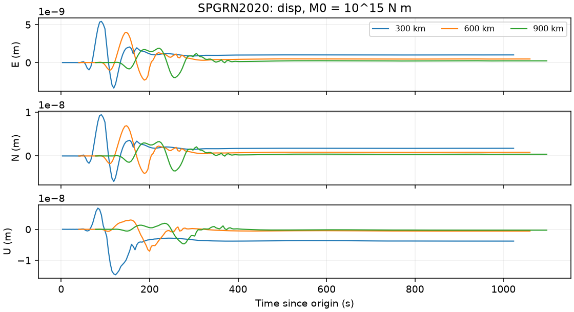
SPGRN2020 displacement plotted in seconds since source origin. — Displacement in metres versus seconds since source origin. Each trace’s start time comes from its native binary record header.#

Outputs are under examples/output/spgrn2020/. disp.npz contains three distances, E/N/up channels, 256 samples per trace and the plotted time coordinates; the summary records the run.

Parameter choices#

spec_time_window=4092 s exceeds time_window=1020 s. The 4 s sample interval, 0.125 Hz cutoff and 64 s source duration define this small long-period calculation. Source duration is in seconds. The example selects spheroidal and toroidal modes, disables the configured self-gravitation range and uses cal_gf=1 for new spectra.

max_slowness=0 selects SPGRN2020’s existing full-wavefield branch, which chooses a model-dependent slowness limit and a larger low-frequency harmonic baseline. It does not restrict the calculation to zero slowness. The previous positive cutoff of 0.3 s/km underestimated the required low-frequency content at 300 km in this example. See the archived 64 s comparison for the evidence and the scope of the revised setting.

green_before_p=40 requests a window beginning approximately 40 s before direct P. The wrapper writes its negative as the Fortran start-time offset; Fortran rounds the resulting start time to the nearest integer second. The example reads that value from each native record header and plots t_start + np.arange(n_samples) * 4 seconds since source origin. The three starts are 3, 40 and 78 s. Simply adding fractional P-table onsets to a -40 s plotting axis would not reproduce those stored starts.

dist_range and delta_dist_range are in km. The backend can choose distance-dependent spacing; use the generated dist_list rather than assuming every request was stored exactly. Recompute spectra if the model, spectral sampling, frequency/slowness cutoffs or mode settings change.

Outputs and reading#

GreenSpec/ holds spectra and GreenFunc/ holds the basis waveforms, GreenInfo*.dat and native tptable.dat/tstable.dat. The metadata update after calculation records dist_list and samples_num.

seek_spgrn2020 returns displacement, velocity or acceleration, with nearest or trilinear interpolation. It synthesizes from ten elementary velocity traces and returns E/N/up by default. The travel-time dictionary also exposes P/S takeoff angles in degrees and native slowness in s/m. Multiply slowness by 1000 for s/km. It is neither the input cutoff’s s/km convention nor TauP ray parameter in s/radian.

The module also contains a cache and a precompute/fast-reader path for repeated queries. Use the main reader as the reference while validating a repeated-query optimization, including cache lifetime and timing options.

Limits and comparison#

The storage window remains referenced to P even though the example now plots source-origin time. Compare backends using the saved time coordinates, matching source, model, units and processing. Raw sample indices do not identify the same physical time across these libraries.

The revised example was checked against QSSP2020 at these three distances and this frequency band. Agreement is a numerical cross-check, not an absolute reference solution or validation for other depths, distances or frequencies. Native Fortran binary metadata must be read with the matching package reader; do not treat it as headerless travel-time arrays.