Comparing backend waveforms

This report records the fresh 15 September 2026 comparison of QSEIS06, QSEIS2025, SPGRN2012, SPGRN2020 and QSSP2020 displacement, together with QSEIS2025/QSSP2020 six-component stress. Every library was newly computed for one source depth and one receiver depth; no existing Green’s libraries were reused. 中文结果说明.

With a common point source, temporal STF and bandwidth, the three spherical backends agree closely. QSEIS06 and QSEIS2025 produce exactly equal saved displacement arrays when their Gaussian wavenumber smoothing settings match. Small timing differences remain between QSEIS and the spherical results.

Note

This calculation uses 2 Hz, a 1.25 s STF and a 1 km receiver depth. The standard regional tutorial scripts retain their lighter 0.125 Hz, 64 s STF, surface-receiver protocol, documented in the earlier comparison. The QSEIS06 point-source result below is an isolated control build, not the default released executable. QSEIS06 and SPGRN2012 remain deprecated.

Common physical and frequency settings

The component overlays follow the presentation of Zhou et al. (2026), DynCFS, Fig. 3. The paper’s figure uses a 10 km distance. This calculation extends its source setup to 300, 600 and 900 km and includes five-backend displacement; it is not a literal reproduction of that figure.

Setting	Fresh calculation
Model	AK135-FC, including depth-dependent Qp/Qs
Source / receiver depth	10 / 1 km
Surface distances / receiver azimuth	300, 600, 900 km / 20°
Strike, dip, rake	223°, 47°, 131°
Scalar moment	3.112616e16 N m, from 2600 * 3460**2 Pa * 1 km² * 1 m, approximately Mw 4.93
Sampling interval / native FFT count	0.25 s / 2048
Requested record span / FFT period	511.75 s / 512 s
Maximum frequency / Nyquist	2 Hz in all five versions
Frequency spacing	1/512 = 0.001953125 Hz
Last retained frequency / Nyquist endpoint	1.998046875 Hz / endpoint at 2 Hz set to zero
Moment-rate STF	Unit-area sin² pulse on 0–1.25 s; centroid 0.625 s
Free surface / physical dispersion / gravity	Included / disabled / disabled
Spherical slowness / harmonic controls	SPGRN max_slowness=0 (full wavefield); QSSP min_harmonic=2000, max_harmonic=40000, max_slowness=0.4
Anti-aliasing factor	0.01
Comparison time grid	Earthquake-origin time 0–400 s, dt = 0.25 s, 1601 samples
Display low-pass	Fourth-order Butterworth at 0.4 Hz, applied forwards and backwards

The model file has SHA-256 de5ec108f9a2e9c54ea3b5a1293e0fba74fdd85ac81856367cb6a7921283ce12. Spherical calculations use all 138 numeric rows. QSEIS uses the identical upper 40 rows, down to 1601.5 km, with Earth flattening. This differs from the lightweight tutorials’ illustrative constant-Q profile.

The QSEIS wrapper converts nominal surface distances using the receiver radius; its native distances are approximately 299.952912, 599.905823 and 899.858735 km. These conventions are retained without fitting distances. Flattening, deep model extent and layered versus spherical geometry remain different numerical approximations.

The paper specifies a 0.4 Hz display low-pass but not its order or phase. This report chooses SciPy sosfiltfilt with default odd-reflection padding on each complete native record before selecting 0–400 s. The two-pass amplitude is one half at 0.4 Hz (−6.02 dB). Display filter, solver cutoff and STF spectrum are distinct.

Displacement at 300, 600 and 900 km

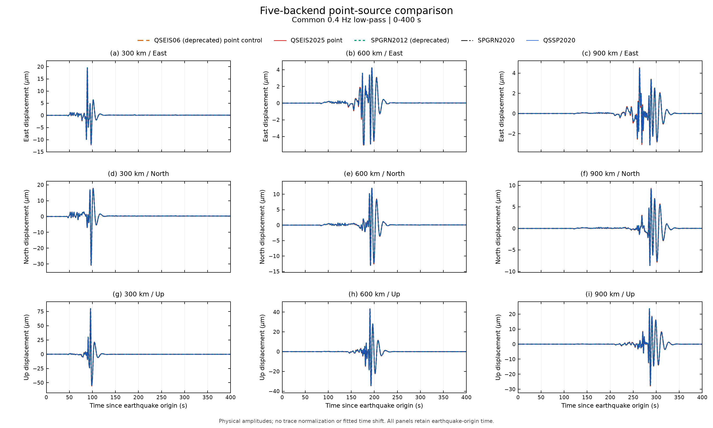
Fresh point-source displacement with the common 0.4 Hz low-pass, in micrometres. QSEIS06 uses the isolated zero-smoothing control build.

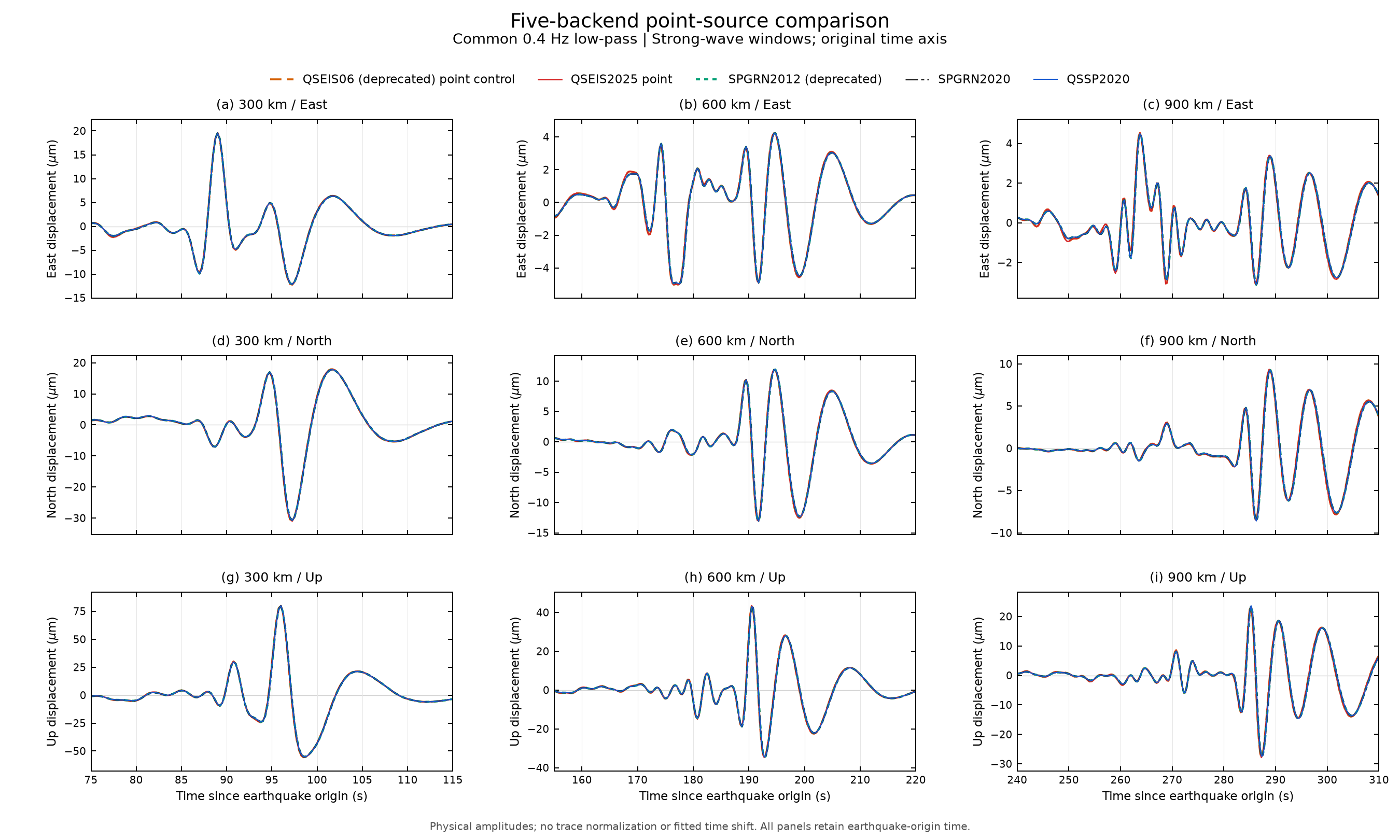
Strong-wave windows on the original time axis. QSEIS06 and QSEIS2025 point-source traces coincide. Main metrics use the full 0–400 s record.

Displacement components are East, North, Up. Arrays and metrics use metres; figures convert to micrometres. All curves retain physical amplitudes, with no fitted time shift, amplitude scale, trace normalization or baseline removal.

The displacement reference is SPGRN2020, not an asserted exact solution. Relative L2 combines all components without rescaling:

\[ E_{L2}=100\sqrt{\frac{\sum_{c,t}(u_c(t)-u_{c,\mathrm{ref}}(t))^2} {\sum_{c,t}u_{c,\mathrm{ref}}(t)^2}}. \]

Displacement versus SPGRN2020, 0.4 Hz low-pass	300 km	600 km	900 km
QSEIS2025, point source	3.5359%	6.8425%	10.6452%
QSEIS06, isolated point-source control	3.5359%	6.8425%	10.6452%
SPGRN2012	0.0054%	0.0102%	0.0143%
QSSP2020	0.2751%	0.2585%	0.2802%

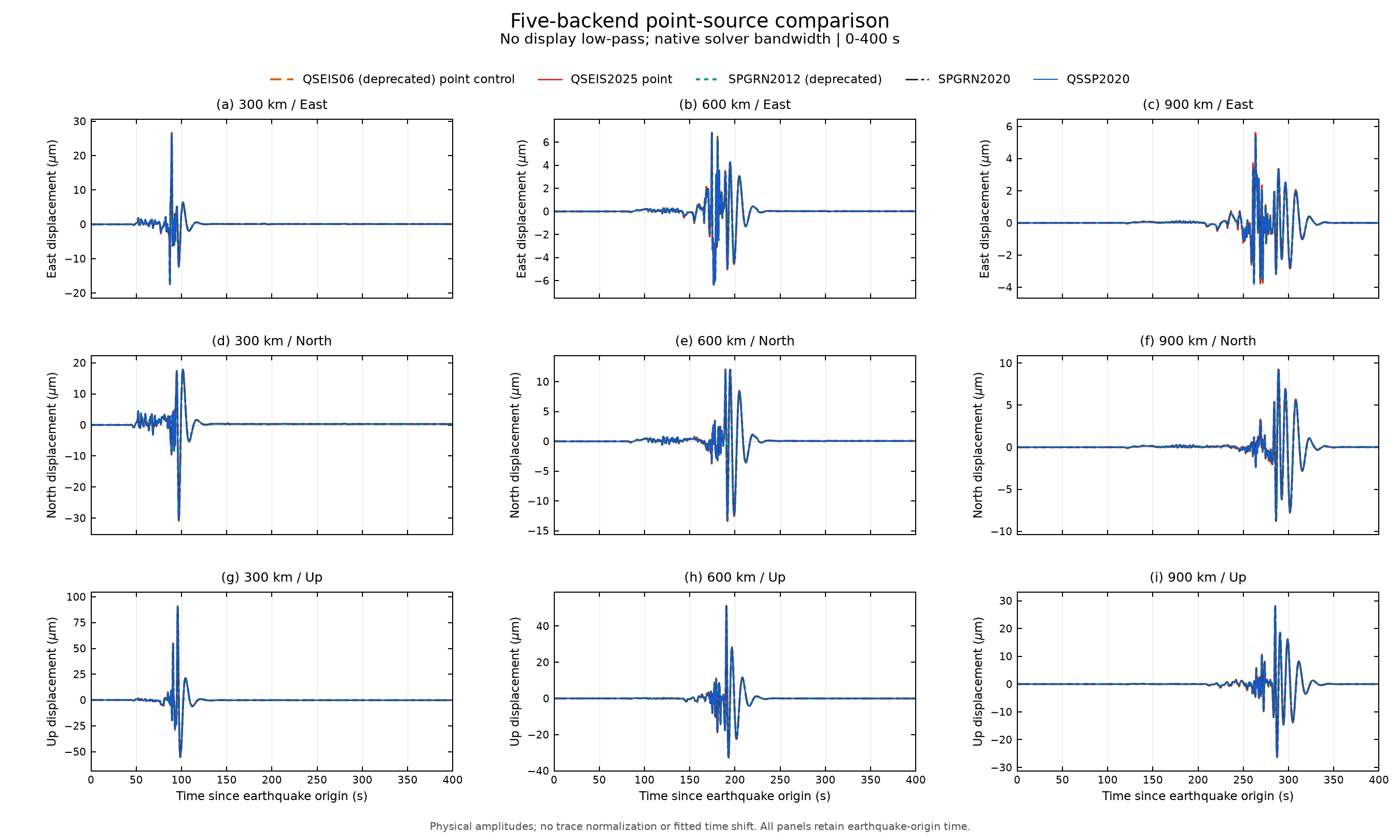
Without the display low-pass, QSEIS2025 displacement L2 values are 3.8480%, 7.3298% and 11.2200%. See the unfiltered displacement figure. Here unfiltered/raw means after the common STF and continuous integration, but before the display low-pass, not unmodified native displacement.

Six-component stress

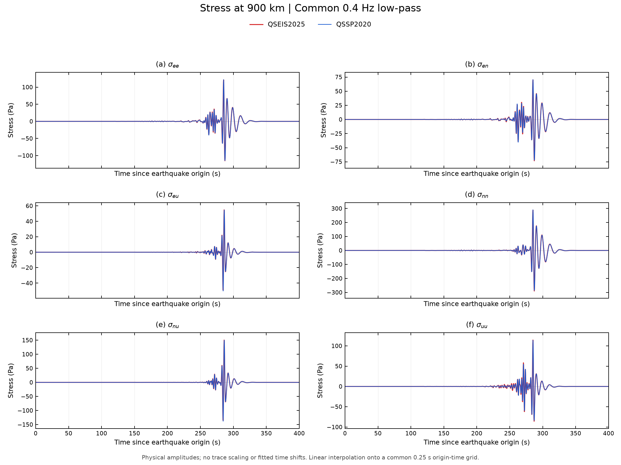
Stress uses [EE, EN, EU, NN, NU, UU] in ENU, in Pa, with tension positive. Shear entries are tensor components, with no engineering factor of two. Reader rotations, signs and component orders were checked against the implementation.

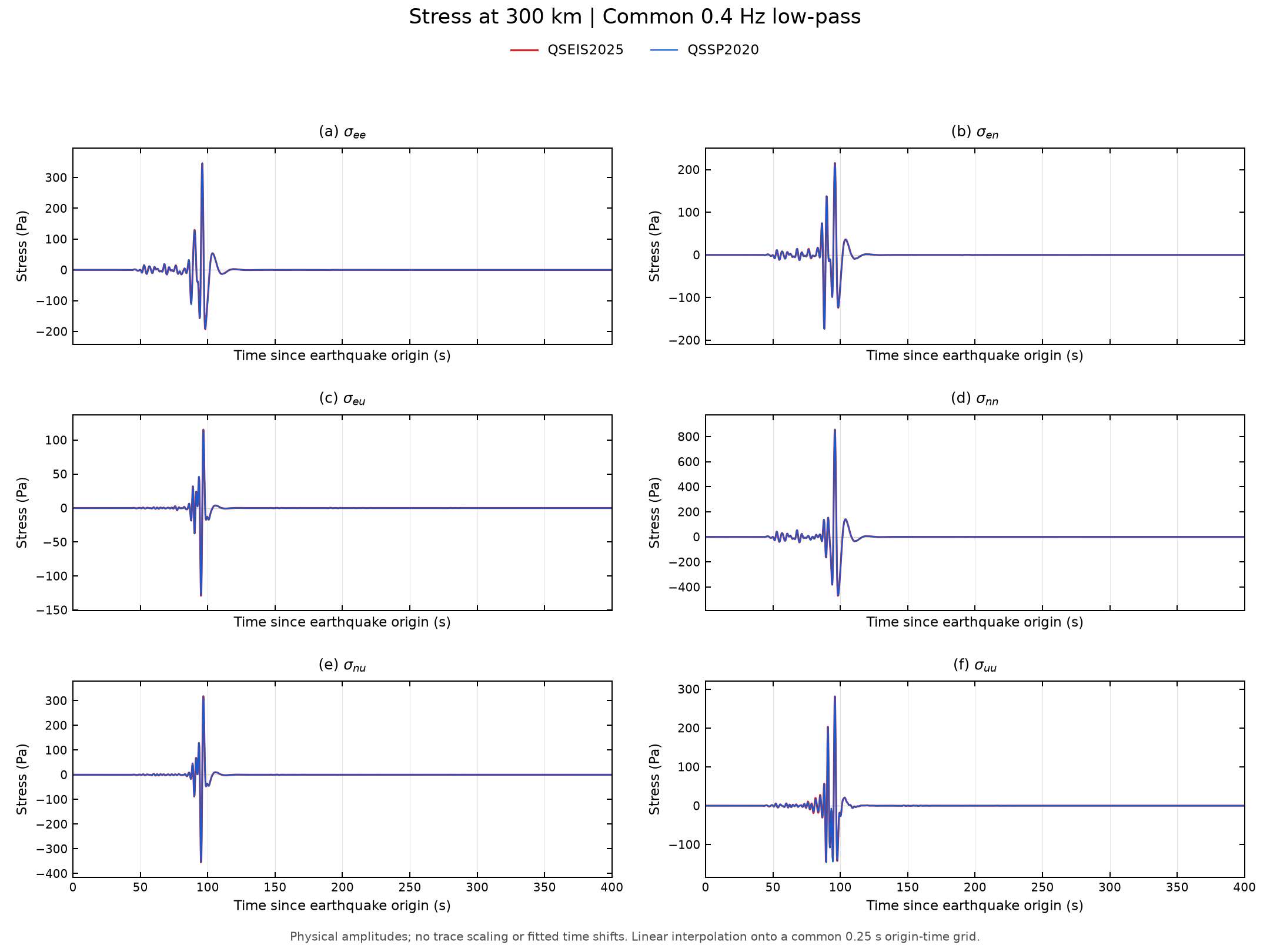
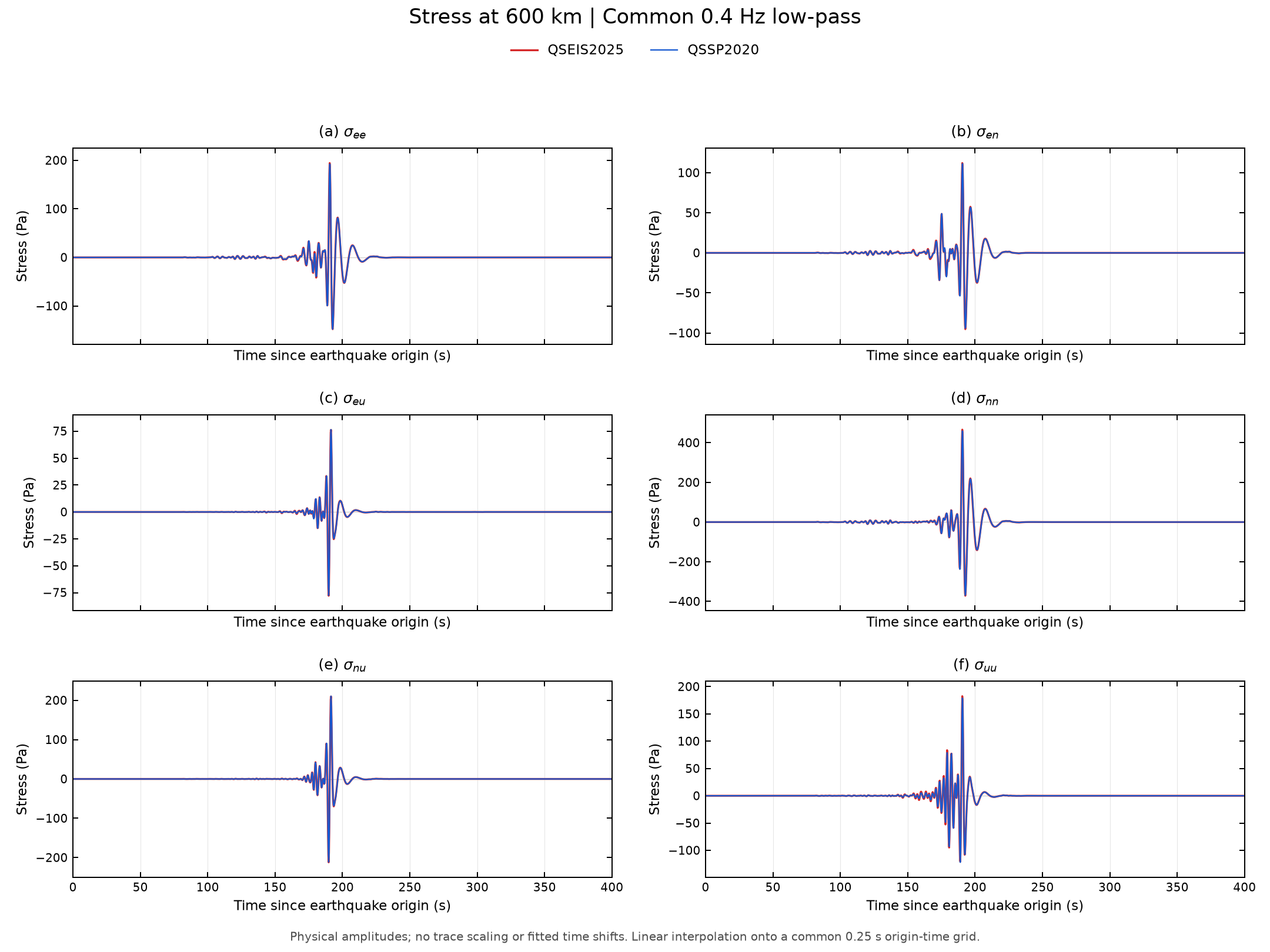
QSSP2020 is the stress reference. L2 includes phase, shape and amplitude differences; it is not a percentage difference of peak stress. The printed Eq. (14) in DynCFS omits the square root; that energy misfit is also saved as (E_L2 / 100)**2.

QSEIS2025 stress versus QSSP2020, all six components	300 km	600 km	900 km
Common 0.4 Hz low-pass	4.2382%	8.2105%	12.5001%
No additional display low-pass	6.7419%	11.8891%	16.1117%

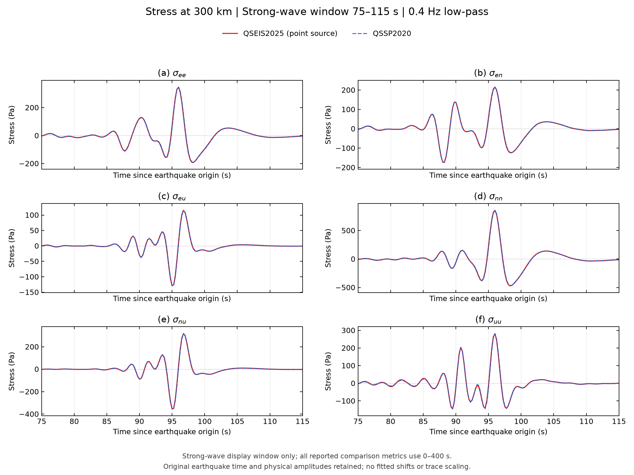
300 km: the 75–115 s window enlarges the strong waves. The reported metric uses 0–400 s; time and amplitude are not fitted.

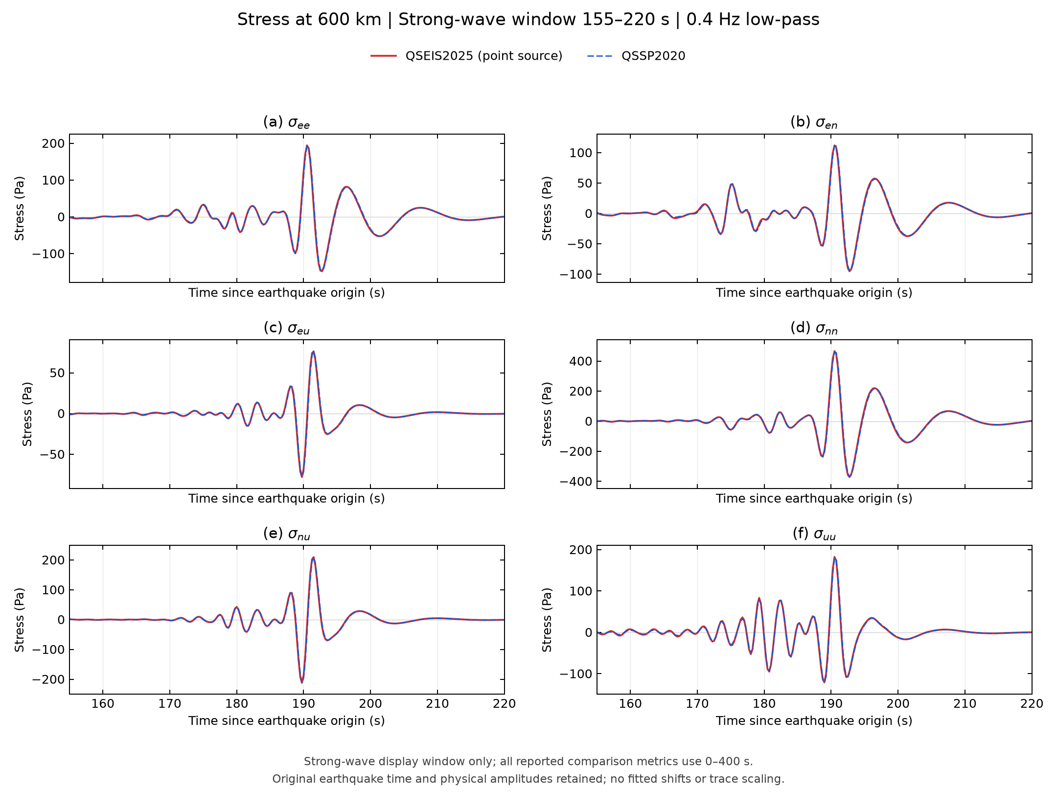
600 km: strong-wave stress comparison over 155–220 s.

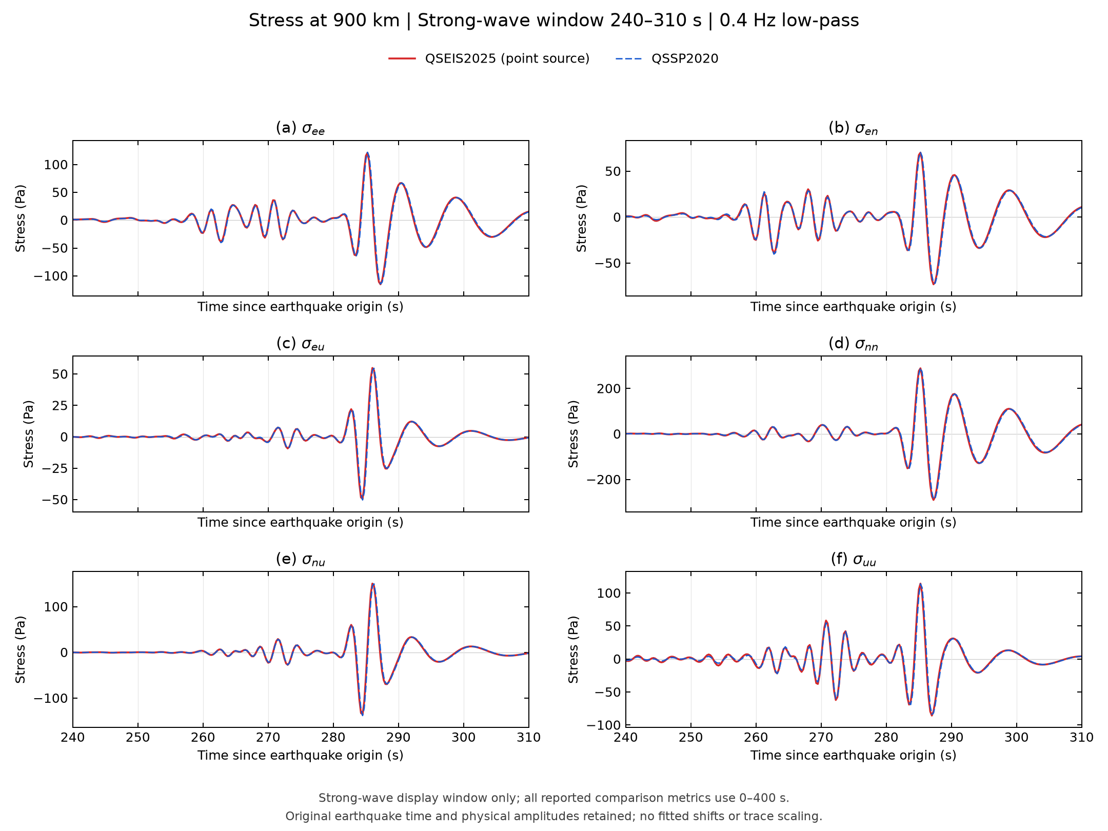
900 km: small timing differences remain despite closely matching peak scales. This view uses 240–310 s, without cropping the underlying metric record.

Full-window stress figures are also available for 300 km, 600 km and 900 km. Downloads contain both processing modes.

QSEIS Gaussian smoothing controls

QSEIS06 hard-codes rd2r=0.05 in qswvint.f. QSEIS2025 exposes it as source_radius_ratio. The wavenumber kernel contains

\[ G(k,f,d)=\exp[-\tfrac12(k a)^2],\qquad a=\rho\min\left[\sqrt{d^2+(z_s-z_r)^2},\frac{v_{P,s}}{f+df}\right], \]

where rho is the radius ratio and the other quantities use the native working model, including flattening where enabled. This frequency-dependent Gaussian wavenumber smoothing is separate from the temporal STF; it is not a fixed-radius finite rupture. The ratio also enters automatic wavenumber-limit estimation, so changing it alters that numerical choice as implemented.

Two fresh controls isolate version and radius settings:

• Ratio 0.05: QSEIS06 and QSEIS2025 saved displacement arrays are bit-identical over all 3 × 3 × 2048 samples.

• Ratio 0: QSEIS06’s isolated control build and QSEIS2025 again produce bit-identical saved displacement arrays over the complete native record.

The QSEIS06 control changes the hard-coded ratio in a copied build. It does not change the installed executable, released default, package API or standard tutorial script. QSEIS2025 accepts zero through its existing input.

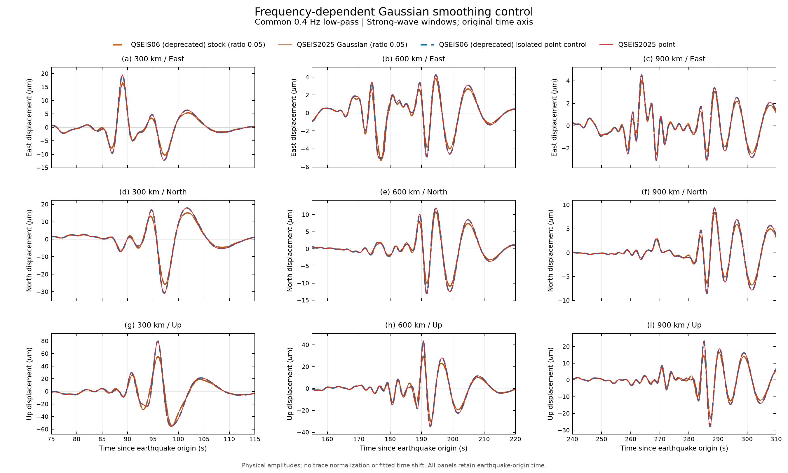
The two versions agree at each matching radius setting. Removing the Gaussian factor changes the waveform while the temporal STF stays fixed.

Common 0.4 Hz low-pass, all displacement components	300 km	600 km	900 km
Ratio 0.05 QSEIS / SPGRN2020	22.8165%	22.3334%	22.7472%
Ratio 0 QSEIS / SPGRN2020	3.5359%	6.8425%	10.6452%
Ratio 0.05 / ratio 0 within the same QSEIS version	22.7849%	21.7443%	20.9496%

This control explains the large separation of the two QSEIS radius configurations in this calculation. It does not identify a unique cause for every discrepancy in earlier libraries.

Matching the effective source time function

The common physical moment rate is

\[ r(t)=\frac{2}{T}\sin^2(\pi t/T),\qquad 0\leq t\leq T,\quad T=1.25\ {\rm s}, \]

and zero elsewhere. QSEIS uses 1024 independent custom source nodes with wavelet_type=0. Values include exp(2*pi*fi*t) to compensate the native inverse transform’s damping correction. Effective area is 1.000000000010, centroid 0.625000002 s and source-spectrum relative L2 error over 0–2 Hz is approximately 1.73e-6.

SPGRN2012 and SPGRN2020 use the zero-duration unit-spectrum branch, then receive the analytic source spectrum on their complete damped FFT records. QSSP2020 evaluates its native 1.25 s sin² source. This is forward convolution, with no source deconvolution or amplitude fitting.

QSEIS uses fi = ln(0.01)/(2*pi*511.75); the spherical backends use fi = ln(0.01)/(2*pi*512). Processing uses each native convention. All rates are integrated on the full damped frequency grid using 1/(2*pi*i*(f+i*fi)), avoiding mismatched rectangular integration rules.

QSSP native export and common integration

For this complete-record configuration, QSSP transfs2t.f exports rates as [x1, ..., xN-1, xN-1], omitting the first FFT sample and duplicating the last. The first sample is recovered uniquely from the native zero Nyquist coefficient; the comparison restores [x0, ..., xN-1] before continuous integration. This deterministic index correction is independent of other backends and is not a fitted arrival-time shift.

Native direct displacement and stress satisfy the exclusive rectangular sum of exported rates, with relative errors below 2.1e-6 in the combined checks. They are preserved in the local calculation archive. The documented waveforms use the common continuous integral and therefore differ from QSSP’s unmodified direct outputs. Downloads record this distinction.

SPGRN2020 native starts are −77, −40 and −2 s; the other comparison records start at zero after documented grid recovery. Filtering precedes selection of the common physical interval. Complete processed native arrays have shape (3, 3, 2048) for displacement and (3, 6, 2048) for stress. Downloads contain the exact 1601-sample arrays used for the figures and main metrics.

Recorded data and verification

The result summary records parameters, platform, runtime/size, hashes and combined results. The data README describes array schemas and baseline versus point-source controls.

Download	Contents
Point-source arrays	Five-backend displacement, including isolated QSEIS06 control
Baseline arrays	Default QSEIS06, point QSEIS2025, spherical displacement, and QSEIS2025/QSSP stress
Radius-control arrays	Both QSEIS versions at ratios 0.05 and 0
Baseline metrics	Component and combined displacement/stress metrics
Point-source metrics	Full-window and strong-wave-window displacement metrics
Radius-control metrics	Within-version and matched-version source controls

All seven result archives passed shape, finite-value, sampling, source and executable-hash checks. The 204 baseline metric rows and 432 point/control rows were recomputed from saved arrays. These checks validate this record; they do not establish convergence for arbitrary Earth models.

The isolated build diffs are available for QSEIS2025 and QSEIS06 point control. Their paths are relative to the repository; they record the separate control builds and are not changes to the released source.

The 2 Hz flattened model exceeded QSEIS’s original lmax=500 capacity, so isolated copies increased it to 2048. Point-source runs partitioned the frequency loop into eight disjoint ranges on the same full FFT grid, then summed high-precision native output columns. Small full-versus-partitioned controls agreed to approximately 3–4e-15 relative L2. Regional frequency coverage, time grids and out-of-band leakage were also checked. The QSEIS06 copy additionally changed the hard-coded radius ratio. These isolated build changes do not alter package defaults. See the validation record.

Replot the documented result

The portable plotting script reads the committed comparison arrays. From the repository root:

python examples/plot_documented_comparison.py --output-dir examples/output/documented-comparison

For arrays before the display low-pass, use --processing raw with a separate output directory. Without a repository checkout, supply --data-dir containing the downloaded point-source-waves.npz and baseline-waves.npz. This needs only NumPy and Matplotlib; it does not run Fortran, Java or a Green’s-function calculation. On Windows with Conda, use conda run -n YOUR_ENV python ....

Replotting reproduces the documented arrays and overlays. Rebuilding the native libraries requires the recorded 2 Hz model, numerical settings and isolated QSEIS controls; ordinary 64 s tutorial commands do not reproduce this new solve. Full native spectra and local calculation logs are not part of the website downloads.