SPGRN2012 (deprecated): reduced-time spherical waveforms#
Deprecated
The SPGRN2012 backend is deprecated in pygrnwang. Use SPGRN2020 for new calculations. This tutorial and its interfaces remain available for existing workflows. Migration requires building a SPGRN2020 library and validating its sampling and time origin; SPGRN2020 uses windows referenced to P instead of SPGRN2012’s reduction rule.
SPGRN2012 computes waveforms for a radially layered spherical Earth. Its
time windows use a reduction offset and velocity, which makes it useful
for reproducing libraries based on t0 + distance / v0.
The fresh comparison dated 2026-09-15 includes a separate SPGRN2012 calculation with 0.25 s sampling, a 2 Hz Nyquist limit, a 1.25 s effective source pulse and receivers 1 km deep. This tutorial keeps its 4 s sampling, 64 s source and surface receivers; its command does not reproduce the new higher-frequency comparison.
Complete calculation#
python examples/spgrn2012.py --output-dir examples/output/spgrn2012-matched-band
The example uses the full Earth model, a 10 km source, surface receivers at approximately 300, 600 and 900 km, and one serial backend job. The actual grid is read from backend metadata after calculation.
"""Deprecated SPGRN2012 tutorial with an explicitly matched physical source.

Retained for existing long-period workflows; use SPGRN2020 for new calculations.
Here the full-period native impulse Green functions are forward-convolved with
the same 64 s moment-rate pulse used by the other regional examples. The reader
then returns displacement from that source-matched library.
"""
from pathlib import Path

import numpy as np

from common import (MECHANISM, MOMENT_NM, REGIONAL_MAX_FREQUENCY_HZ,
                    REGIONAL_SAMPLING_INTERVAL_S, REGIONAL_SOURCE_DURATION_S,
                    REGIONAL_STF, finish, parser_for, prepare,
                    require_library_settings, save_waveforms)
from pygrnwang.create_spgrn2012_bulk import (
    pre_process_spgrn2012, create_grnlib_spgrn2012_sequential)
from pygrnwang.pytaup import create_tpts_table
from pygrnwang.read_spgrn2012 import seek_spgrn2012
from spectral_settings import verify_spherical_spectrum
from spherical_source_time_function import (inspect_spgrn2012_native, save_spgrn2012_stf,
                                           validate_spgrn2012_stf, write_spgrn2012_matched_library)


def main():
    args = parser_for("spgrn2012").parse_args()
    output, library, model, report, started = prepare(
        args, "SPGRN2012", extra={"display_name": "SPGRN2012 (deprecated)"})
    dt, native_window, output_window = REGIONAL_SAMPLING_INTERVAL_S, 4092.0, 1020.0
    t0, v0 = -40.0, 10.0
    output_samples = int(round(output_window / dt)) + 1
    if not args.reuse:
        pre_process_spgrn2012(
            processes_num=1, path_green=library, event_depth_list=[10.0],
            receiver_depth_list=[0.0], spec_time_window=native_window,
            sampling_interval=dt, max_frequency=REGIONAL_MAX_FREQUENCY_HZ, max_slowness=0.0,
            anti_alias=0.01, gravity_fc=0.0, gravity_harmonic=0,
            cal_sph=1, cal_tor=1, source_radius=0.0, cal_gf=1,
            time_window=native_window, t0=t0, v0=v0, source_duration=0.0,
            dist_range=[300.0, 900.0], delta_dist_range=[300.0, 300.0],
            path_nd=model, earth_model_layer_num=None, physical_dispersion=0,
        )
        create_grnlib_spgrn2012_sequential(library)
    info = require_library_settings(
        library, event_depth_list=[10.0], receiver_depth_list=[0.0],
        spec_time_window=native_window, time_window=native_window, sampling_interval=dt,
        samples_num=1024, source_duration=0.0, max_frequency=REGIONAL_MAX_FREQUENCY_HZ,
        max_slowness=0.0, anti_alias=0.01, physical_dispersion=0,
        gravity_fc=0.0, gravity_harmonic=0, cal_sph=1, cal_tor=1,
        source_radius=0.0, t0=t0, v0=v0, dist_list=[300.0, 600.0, 900.0],
    )
    native = inspect_spgrn2012_native(library)
    if args.reuse:
        validate_spgrn2012_stf(library)
    distances = info["dist_list"]
    if not args.reuse:
        # The serial builder does not create these tables; the reader needs them.
        create_tpts_table(str(Path(library) / "GreenFunc"), 10.0, 0.0,
                          distances, info["path_nd_without_Q"], False)
    # Preserve the whole FFT period during source convolution. The reader then
    # integrates all 1024 matched samples; export the first 256 on each trace's
    # actual origin-time axis.
    matched_library, source = write_spgrn2012_matched_library(library, native)
    arrays = np.array([MOMENT_NM * seek_spgrn2012(
        path_green=matched_library, event_depth_km=10.0, receiver_depth_km=0.0,
        az_deg=30.0, dist_km=distance, focal_mechanism=MECHANISM,
        srate=1 / dt, output_type="disp", rotate=True,
        before_p=None, shift=False, pad_zeros=False,
    ) for distance in distances])[:, :, :output_samples]
    save_waveforms(output, report, "disp", arrays, distances, dt,
                   ["E", "N", "U"], "m", start_times=native["trace_start_times_s"],
                   expected_samples=output_samples)
    source = save_spgrn2012_stf(output, native, source)
    validate_spgrn2012_stf(library)
    report.update(sampling_interval_s=dt, time_window_s=native_window,
                  native_samples=1024, output_window_s=output_window,
                  output_time_ranges_s=[[start, start + output_window]
                                        for start in native["trace_start_times_s"]],
                  distances_km=distances, spec_time_window_s=native_window,
                  max_frequency_hz=REGIONAL_MAX_FREQUENCY_HZ,
                  last_retained_frequency_hz=native["last_retained_frequency_hz"],
                  nyquist_bin_zero=True, t0_s=t0, v0_km_s=v0,
                  trace_start_times_s=native["trace_start_times_s"],
                  native_source_duration_s=0.0, source_duration_s=REGIONAL_SOURCE_DURATION_S,
                  effective_source_duration_s=REGIONAL_SOURCE_DURATION_S,
                  physical_source_time_function=dict(REGIONAL_STF),
                  full_wavefield=True, max_slowness_s_km=0.0,
                  source_radius_km=0.0,
                  spectral_settings=verify_spherical_spectrum(library, 'SPGRN2012'),
                  source_time_function=source)
    finish(output, report, started)


if __name__ == "__main__":
    main()
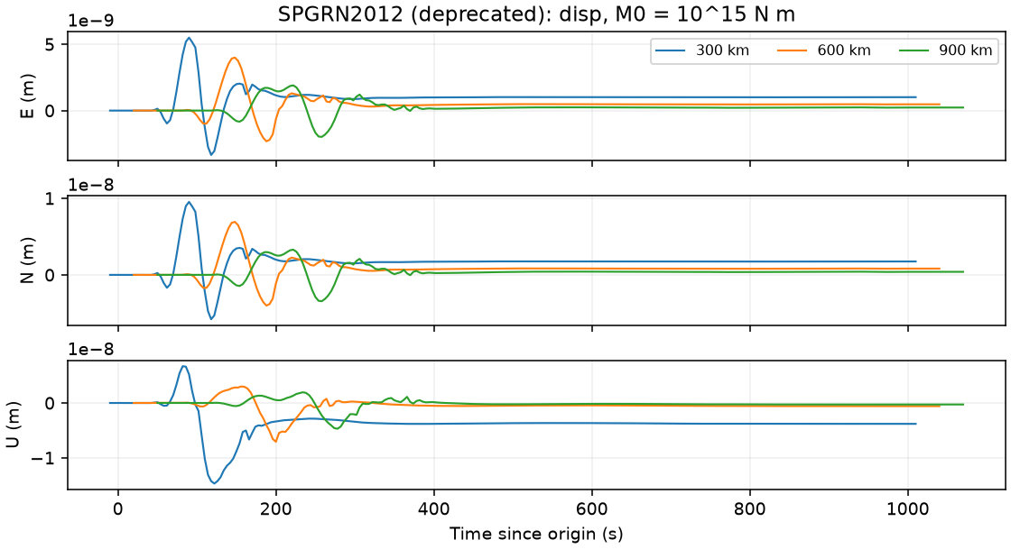
Displacement in metres. Each trace uses its own reduced start time to show time since source origin.#
The command above saves results beneath
examples/output/spgrn2012-matched-band/. disp.npz has shape
(3 distances, 3 ENU components, 256 samples) in metres; disp.png and
summary.json describe the exported result. library/ contains the
native spectral files and impulse Green functions. Two further outputs
make the source calculation inspectable:
library-source-matched/: the same metadata and travel-time tables, with every native Green function forward-convolved with the physical source; the script reads displacement from this library;source_time_function.npzand.json: the physical pulse, its analytic complex-frequency transform, validated native settings and hashes of the matched Green functions and exported displacement.
The script’s default output directory remains
examples/output/spgrn2012/; the explicit directory above keeps this
calculation separate from earlier tutorial runs.
Spectra, output window and source#
Both the spectral window and the native velocity output window are 4092 s, sampled at 4 s. The native FFT has 1024 samples and period 4096 s. The script applies the physical source to all 1024 samples of every Green function. The reader then integrates the complete matched record once, and the script exports the first 256 samples spanning 1020 s. Convolving only the cropped displacement cannot reproduce this operation. Neither can convolving displacement read from the impulse library: that integral of the unfiltered impulse velocity is dominated by drift.
max_frequency=0.125 Hz equals the sampling Nyquist frequency.
The actual spectrum header must contain nfcut=512, with frequency spacing
1/4096 Hz. The solver explicitly zeroes the Nyquist bin, so its highest
computed frequency is 511/4096 = 0.124755859375 Hz.
max_slowness=0 requests the full wavefield. cal_sph=1 and cal_tor=1
include P-SV and SH contributions, and source_radius=0 selects a point
source. gravity_fc/gravity_harmonic and physical_dispersion are zero;
the native additional Butterworth filter is disabled.
The physical source shared with the other regional examples is the unit-area moment-rate pulse
with zero rate outside that interval and centroid 32 s. This tutorial
sets the native source_duration=0, whose spectrum is unity, and
applies the target 64 s source to the Green functions in the example
script. The library metadata
therefore correctly records zero native duration; the summary separately
records native_source_duration_s=0 and effective_source_duration_s=64.
No solver kernel or public reader behavior is changed.
The native imaginary frequency is
fi = log(0.01) / (2*pi*4096). The helper restores the numerical damping
of each complete impulse Green function, transforms it, multiplies by the exact
transform of r(t) at f + i*fi, transforms back and removes damping.
This is forward convolution: there is no division by an existing source
spectrum, fitted amplitude or time shift. The damped DC coefficient is
about 0.9647432; it must not be renormalized because the physical rate
already integrates to one. Independent quadrature checks the analytic
transform across the full 0–0.125 Hz band.
def apply_spgrn2012_stf(velocity, native):
    """Forward-convolve complete physical impulse velocities, retaining their time axes."""
    values = np.asarray(velocity, dtype=float)
    if values.shape[-1] != 1024 or not np.isfinite(values).all():
        raise ValueError("Expected complete, finite 1024-sample velocity records")
    dt = native["fft_header"]["dt"]
    frequency = np.fft.rfftfreq(1024, dt)
    transfer = sin_squared_spectrum(frequency, native["fi_hz"])
    damping = np.exp(2 * np.pi * native["fi_hz"] * np.arange(1024) * dt)
    spectrum = np.fft.rfft(values * damping, axis=-1)
    # The native inverse FFT explicitly sets Nyquist to zero. Remove only any
    # roundoff introduced there by storing the impulse velocity as float32.
    spectrum[..., -1] = 0.0
    matched = np.fft.irfft(spectrum * transfer, n=1024, axis=-1) / damping
    if not np.isfinite(matched).all():
        raise ValueError("Non-finite velocity after forward source convolution")
    # Independent quadrature checks the analytic transform over the whole band.
    nodes, weights = np.polynomial.legendre.leggauss(64)
    times = (nodes + 1) * REGIONAL_SOURCE_DURATION_S / 2
    rate = 2 / REGIONAL_SOURCE_DURATION_S * np.sin(np.pi * times / REGIONAL_SOURCE_DURATION_S) ** 2
    quadrature = (np.exp(-2j * np.pi * (frequency[:, None] + 1j * native["fi_hz"]) * times)
                  @ (weights * rate)) * REGIONAL_SOURCE_DURATION_S / 2
    error = float(np.linalg.norm(quadrature - transfer) / np.linalg.norm(transfer))
    area = float(np.sum(weights * rate) * REGIONAL_SOURCE_DURATION_S / 2)
    if error >= 1e-12 or abs(area - 1.0) >= 1e-12:
        raise ValueError("Analytic source transform failed independent full-band quadrature validation")
    metadata = {
        "scheme_id": SCHEME_ID, "physical_source_time_function": dict(REGIONAL_STF),
        "native_source_duration_s": 0.0, "effective_source_duration_s": REGIONAL_SOURCE_DURATION_S,
        "method": "full-period damped-domain analytic forward convolution of every native impulse Green function",
        "spectral_division": False, "fitted_amplitude": False, "fitted_time_shift": False,
        "native": native, "physical_rate_integral": area,
        "analytic_transform_relative_l2_vs_quadrature": error,
        "damped_dc_coefficient": float(transfer[0].real),
        "matched_library": MATCHED_LIBRARY,
        "integration": "seek_spgrn2012(output_type='disp') integrates all 1024 matched samples; "
                       "the example then retains the first 256",
    }
    return matched, metadata
cal_gf=1 requests spectral calculation. delta_dist_range gives the
smallest/largest distance increments in km; equal values request a uniform
grid. The script reads the actual dist_list from green_lib_info.json.
Fortran rounds t0 + distance / v0 to the nearest integer second for
the native start time. Here t0=-40 s and v0=10 km/s, giving starts
of -10, 20 and 50 s. The saved displacement axes therefore cover
-10–1010, 20–1040 and 50–1070 s relative to source origin. SPGRN2020
uses a different start rule based on P onset; compare their traces only
over the shared origin-time interval.
Use --reuse with the same explicit output directory only after a
successful run. The script checks native input records, all spectral
headers, complete velocity blocks, the physical pulse and archive hashes,
and recomputes the matched Green functions from the native library.
Older libraries with a native 64 s source, a 0.0625 Hz cutoff, a slowness
limit or a cropped native output are rejected and require a fresh build.
Travel-time tables are part of the workflow#
The sequential builder updates library metadata but does not create the
Python travel-time tables consumed by seek_spgrn2012.
The script explicitly runs create_tpts_table after construction, using
the generated noQ.nd and backend’s actual distance grid.
Keep the resulting tp_table.bin/ts_table.bin beneath the depth pair in
GreenFunc/. The reader loads them even when shift=False.
A successful Fortran run alone is therefore insufficient for a complete
Python-readable SPGRN2012 library.
Reading and limits#
The raw basis library represents velocity. In the general reader,
output_type="disp" integrates it and "acce" differentiates it.
This example reads the source-matched library with output_type="disp",
so the reader applies cumsum * dt exactly once. It scales a
unit mechanism by 10^15 N m and returns E/N/up components. Nearest and
trilinear waveform interpolation remain available in the reader.
Earlier tutorial comparisons reported approximately 4% differences from SPGRN2020. Those results used a different frequency cutoff and SPGRN2012’s native real-frequency wavelet, whose effective area became about 3.67% larger after damping correction. They are historical results, not a characterization of the source-matched example above. See the archived 64 s comparison for the source-matched tutorial, measured differences and remaining model/sampling limitations. Matching the physical source and requested frequency band does not establish exact equivalence between the solvers.
The 64 s source and coarse distance grid do not establish convergence for high-frequency regional phases or other source/receiver geometries. Compare unshifted grid-point traces first, then validate interpolation or arrival-based waveform adjustments for your application.