Wenchuan earthquake

This example uses a finite-fault model of the 2008 Wenchuan earthquake. The model has five source planes with a total scalar moment of 1.04 × 10²¹ N m (Mw 7.95). It runs two calculations:

1. Stress history on a receiver fault. Source plane 4 loads plane 5. The example computes quasi-static and dynamic CFS as the rupture grows.

2. Static CFS map at 15 km depth. All five planes load a geographic grid. The map is computed in a layered model and in a homogeneous half-space.

The input data and the original scripts are in examples/wenchuan/.

Input model

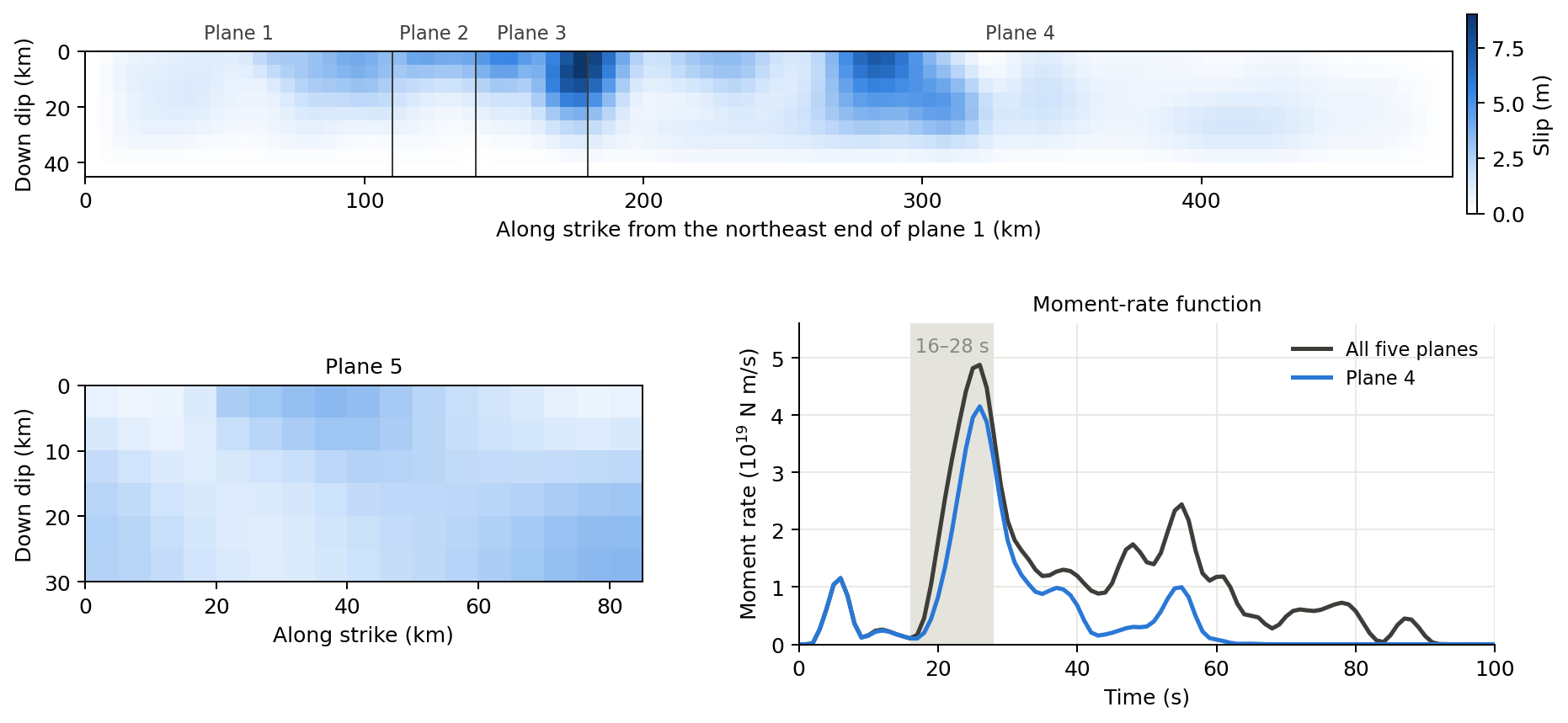
Planes 1–4 lie end to end along strike and share the same depth range. The top panel shows them from the northeast end of plane 1, with distance measured down dip from the top edge. Plane 5 is a separate, shallower fault. The moment-rate function combines all five planes; plane 4 dominates the main pulse between about 16 and 28 s.

Plane	Patches (strike × dip)	Patch size	Strike	Dip	Peak slip
1	22 × 9	5 × 5 km	228°	10–40°	4.07 m
2	6 × 9	5 × 5 km	223°	10–40°	4.23 m
3	8 × 9	5 × 5 km	218°	10–40°	9.03 m
4	62 × 9	5 × 5 km	225°	10–40°	8.31 m
5	17 × 6	5 × 5 km	223°	25–65°	3.53 m

Dip varies with depth on every plane. Rake varies patch by patch, and each patch has a 240-sample source time function at 0.5 s. obs_plane5.csv repeats the geometry of plane 5 and supplies a receiver rake for each cell. The Earth model is input/model.nd.

Stress history on plane 5

Setting	Value
Source	Plane 4 only; patches with slip below 1 m are ignored (slip_thresh = 1)
Receiver	Plane 5, 17 × 6 cells, mechanism of each cell from obs_plane5.csv
Friction / Skempton coefficient	0.4 / 0
Static library	Source depths 1–31 km (2 km), distances 0–800 km (2 km)
Dynamic library (QSEIS2025)	Source depths 1–31 km and receiver depths 0–32 km (2 km); distances 2–1000 km (2 km)
Time sampling	STF and CFS at 0.5 s; 1024 samples (0–511.5 s)

Quasi-static CFS at time t uses the slip accumulated up to t: it keeps the first cut_stf = 2t STF samples (cut_stf = 0 means the final slip). Dynamic CFS includes the transient seismic waves.

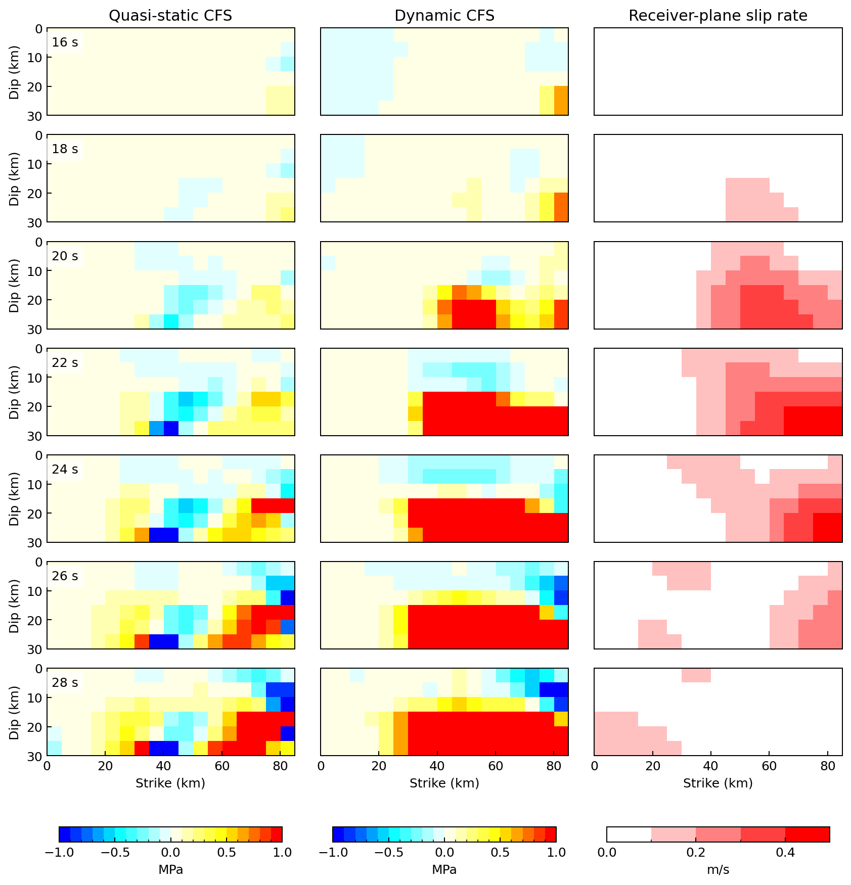
Each row is one time between 16 and 28 s. The two CFS columns share the −1 to +1 MPa scale with 0.1 MPa bins. The right column shows the slip rate of plane 5 from its own input source time function. Plane 5 is not a source in this calculation; the column shows when that fault slipped.

Dynamic CFS rises faster than quasi-static CFS. On the lower half of plane 5 (more than 15 km down dip), dynamic CFS exceeds +1 MPa on about half of the cells from 22 s. Quasi-static CFS exceeds +1 MPa on at most 16% of those cells by 28 s. In this window, slip rate on plane 5 first exceeds 0.1 m/s at 18 s. Final static CFS on plane 5 ranges from −5.58 to 3.91 MPa. Dynamic CFS ranges from −2.97 to 26.42 MPa over the full time series.

Static CFS map at 15 km

Setting	Value
Sources	Planes 1–5 (984 patches), slip_thresh = 1
Receivers	15 km depth; latitude 28.5–34.5°, longitude 101–107°, 0.01° spacing (601 × 601 points)
Receiver mechanism	Strike 223°, dip 47°, rake 131°
Friction / Skempton coefficient	0.4 / 0
Static libraries	Source depths 0–30 km (1 km), distances 0–1000 km (1 km), receiver depth 15 km
Half-space elasticity	λ = 25.21168 GPa, μ = 31.12616 GPa

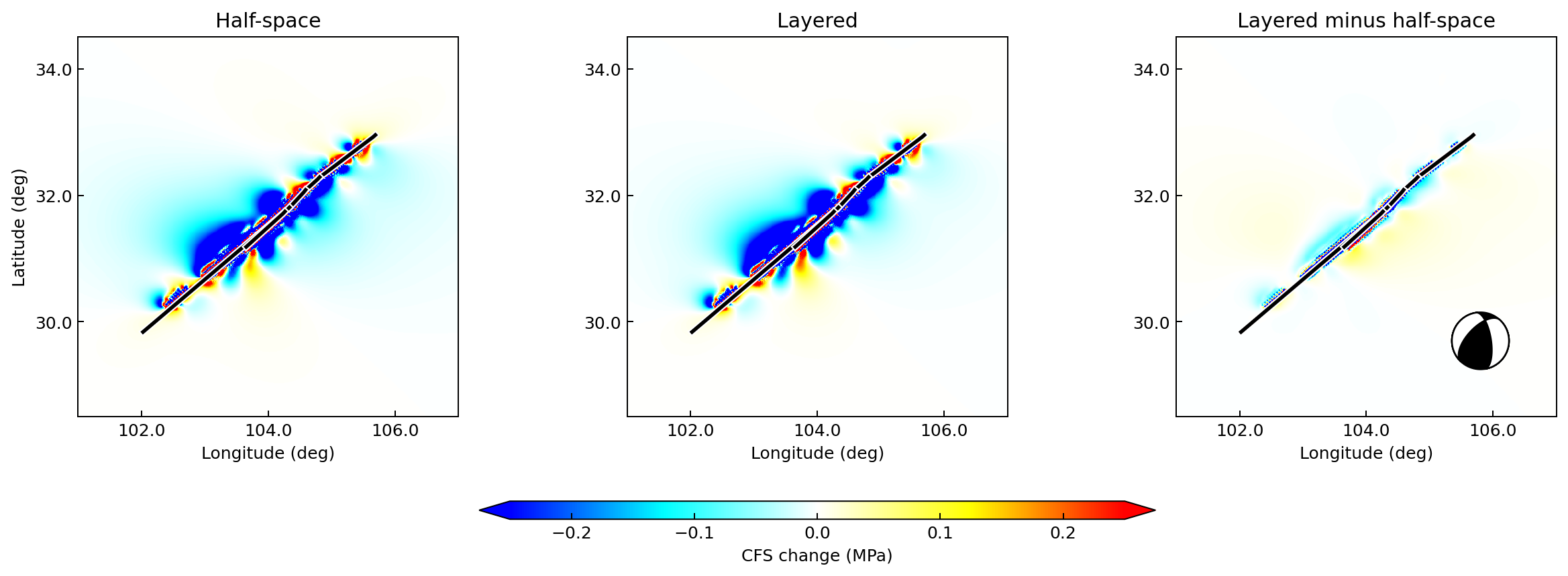
All three panels use ±0.25 MPa; stronger values are saturated. The black line marks where the source planes cross 15 km depth. The half-space and layered maps show the same pattern of positive and negative lobes. Their difference is concentrated next to the fault: more than 25 km from the nearest source patch it stays below 0.04 MPa, and beyond 100 km below 0.015 MPa. Map CFS ranges from −768.5 to 352.5 MPa in the half-space and from −781.6 to 332.1 MPa in the layered model. These extremes lie within about 1 km of a source patch.

Run the example

The documentation runner copies the inputs, sets absolute paths in a copy of the INI and writes everything to docs/_build/cases/wenchuan/. Run it from the repository root:

conda run -n pygrnwang python docs/examples/run_case_studies.py --case wenchuan
conda run -n pygrnwang python docs/examples/plot_case_inputs.py
conda run -n pygrnwang python docs/examples/plot_case_studies.py --figure wenchuan-plane
conda run -n pygrnwang python docs/examples/plot_case_studies.py --figure wenchuan-static

The calculation needs EDGRN2, EDCMP2, QSEIS2025 and Java/TauP. The runner has three stages: --stage static, --stage dynamic-library and --stage dynamic. A completed stage is skipped; add --force-stage to repeat it. Use a new --output-dir after changing inputs or grid spacing. With 12 worker processes, the stages took about 7 min, 2 h and 30 s. The runner builds only the library depths and distance groups that the receivers query, so its libraries are smaller than the INI ranges.

The original scripts can also be run directly. First replace the /e/dyncfs_data/ paths in wenchuan.ini.

Script	Purpose
compute_cfs_static_along_time.py	Static library and quasi-static CFS on plane 5 for cut_stf = 0, 2, …, 78
compute_dynamic_cfs.py	Dynamic library and dynamic CFS on plane 5
compute_static_cfs_fix_depth.py	Layered static map at 15 km
compute_cfs_static_half_space_fix_depth.py	Half-space static map at 15 km
plot_plane5_compare_2d.py, plot_compare_static_cfs_fix_dep.py	Plot the two calculations
plot_slip_3d_wenchuan.py	3D slip view; also reads stf.npy, which is not included
create_coulomb3.py	Export the sources to a Coulomb 3 input file

Before running the original map scripts, note:

• wenchuan.ini selects source plane 4. The map scripts switch to planes 1–5 in code.

• The map scripts set the grid spacing to 0.05°, while the INI uses 0.01°. The figures above use 0.01°.

• source_shapes in the map scripts has one extra level of nesting. Write it as [[22, 9], [6, 9], [8, 9], [62, 9], [17, 6]].

• create_static_lib is commented out in the layered map script, and the half-space script never builds a library. Build a library with matching layered, lam and mu settings before computing.

• The half-space script reads its INI from an absolute path; change it to your copy of wenchuan.ini.

• The full map has 361 201 receivers. Start with a coarser grid when testing.

create_coulomb3.py converts the selected geometry for Coulomb 3. It writes the input file but does not run Coulomb 3.

Output files

Under docs/_build/cases/wenchuan/results/:

Path	Content
static/cfs_static_plane5.csv	Final static CFS on the 102 cells of plane 5 (Pa)
static/time/<cut_stf>/cfs_static_plane5.csv	Quasi-static CFS for each STF cutoff
dynamic/cfs_dynamic_plane5.csv	Dynamic CFS, 102 rows × 1024 samples (Pa)
static_layer/, static_half/	Maps at 15 km: cfs_static_dep_15.00.csv and the stress tensor stress_tensor_dep_15.00.npy

Each map CSV has one value per grid point, with longitude varying fastest. run.json records input hashes, program versions, stage timings and result statistics.