Ludian earthquake

This example uses a finite-fault model of the 3 August 2014 Ludian earthquake in Yunnan. The model has two intersecting source planes with a total scalar moment of 2.13 × 10¹⁸ N m (Mw 6.15). The example computes static and dynamic Coulomb stress changes on optimally oriented planes at 5 km depth and plots them with the aftershock catalog.

The input data and the original scripts are in examples/ludian/.

Input model

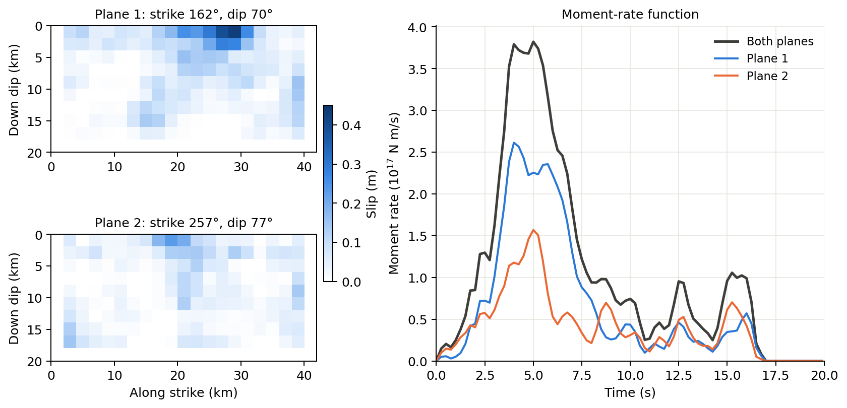
Distance along strike starts at the first row of each CSV file; distance down dip starts at the top edge. About three quarters of the moment is released in the first 8 s, with later pulses at about 12.5 and 15.5 s. Plane 1 carries the larger slip.

Plane	Patches (strike × dip)	Patch size	Strike	Dip	Depth	Peak slip
1	21 × 10	2 × 2 km	162°	70°	0.9–17.9 km	0.43 m
2	21 × 10	2 × 2 km	257°	77°	1.0–18.5 km	0.23 m

Rake varies patch by patch. Each patch has a 160-sample source time function at 0.125 s. The Earth model is input/model.nd. after_ludian.txt lists 976 events from 3 to 19 August 2014 as longitude, latitude, depth and magnitude; after_time.txt gives their times.

Calculation settings

Setting	Value
Sources	Planes 1 and 2 (420 patches); slip below 0.1 m is ignored (slip_thresh = 0.1)
Receivers	5 km depth; latitude 26.9–27.3°, longitude 103.2–103.6°, 0.01° spacing (41 × 41 points)
Receiver orientation	Optimally oriented planes (optimal_type = 2)
Regional stress axes (azimuth / plunge)	Most compressive 130.60° / 4.63°; intermediate 16° / 79°; least compressive 221.41° / 9.96°
Friction / Skempton coefficient	0.6 / 0.75
Static library	Source depths 1–20 km (0.5 km), distances 0.25–150 km (0.25 km)
Dynamic library (QSEIS2025)	Source depths 1–20 km and receiver depths 0.25–20.25 km (0.5 km); distances 0.25–150 km (0.25 km)
Time sampling	STF and CFS at 0.125 s; 1024 samples (0–127.875 s)

With a nonzero Skempton coefficient, CFS includes the mean-stress term:

\[\Delta CFS = \Delta\tau + \mu_f(\Delta\sigma_n - B\,\Delta\sigma_m).\]

The regional stress axes set the orientation of the optimal planes; the reported CFS is the stress change caused by the earthquake. See the receiver modes for details.

Receiver depths in the library are 0.25, 0.75, … km. The static reader takes the nearest depth, 4.75 km, for the requested 5 km. Dynamic synthesis interpolates between 4.75 and 5.25 km. Some patches of both planes are shallower than the 1 km library limit; their queries use the 1 km boundary.

Results

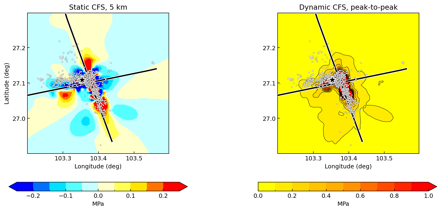
The left panel shows static CFS on a −0.25 to +0.25 MPa scale with 0.05 MPa bins. The right panel shows the peak-to-peak dynamic CFS on a 0–1 MPa scale with 0.1 MPa bins and contours:

\[\max\bigl(0,\max_t\Delta CFS(t)\bigr)-\min\bigl(0,\min_t\Delta CFS(t)\bigr).\]

Black lines mark where the planes cross 5 km depth. White dots are the catalog events; the star is the first event, the mainshock. The panels are displayed with fivefold bilinear interpolation of the 41 × 41 grid.

Static CFS ranges from −4.17 to 7.48 MPa. Dynamic CFS ranges from −6.82 to 25.00 MPa over the time series, and its peak-to-peak value from 0.016 to 25.03 MPa. Positive static CFS covers 36% of the map, and 60% of the 967 events inside the map fall there. Peak-to-peak dynamic CFS of at least 0.1 MPa covers 18% of the map and 87% of those events. The maps are at 5 km, whereas the median event depth is 9.7 km, so these fractions only describe the map-view pattern.

Run the example

The documentation runner copies the inputs, sets absolute paths in a copy of the INI and writes everything to docs/_build/cases/ludian/. Run it from the repository root:

conda run -n pygrnwang python docs/examples/run_case_studies.py --case ludian
conda run -n pygrnwang python docs/examples/plot_case_inputs.py
conda run -n pygrnwang python docs/examples/plot_case_studies.py --figure ludian

The calculation needs EDGRN2, EDCMP2, QSEIS2025 and Java/TauP. The runner has three stages: --stage static, --stage dynamic-library and --stage dynamic. A completed stage is skipped; add --force-stage to repeat it. Use a new --output-dir after changing inputs. With 12 worker processes, the stages took about 20 s, 12 min and 9.5 min. The runner builds only the library depths and distance groups that the receivers query.

The original scripts can also be run directly:

File	Purpose
compute_static_and_dynamic_cfs_fix_depth.py	Build both libraries and compute static and dynamic CFS at 5 km
plot_compare_cfs_oop_fix_dep.py	Plot static and peak-to-peak dynamic CFS with aftershocks

Replace the /e/dyncfs_data/ paths in ludian.ini first. The script reads ludian.ini from the current directory and runs dynamic synthesis in parallel; keep its if __name__ == "__main__": guard (see parallel runs). The original plotting script computes the grid size with an unrounded ceil, which can give 42 points instead of 41; plot_case_studies.py uses cal_grid_num instead.

Output files

Under docs/_build/cases/ludian/results/:

Path	Content
static/cfs_oop_static_dep_5.00.csv	Static CFS, 1681 values (Pa)
static/stress_tensor_dep_5.00.npy	Static stress tensor, (1681, 6), NED components (Pa)
dynamic/cfs_oop_dynamic_dep_5.00.csv	Dynamic CFS, 1681 rows × 1024 samples (Pa)

Grid points are ordered with longitude varying fastest. Normal vectors, slip directions and normal and shear stresses are saved for both conjugate planes; the CFS files use the second plane. run.json records input hashes, program versions, stage timings and result statistics.